A synthetic bayesqm_fit for examples and tutorials

Returns a bayesqm_fit with realistic Q-methodology structure: every participant has a dominant factor, roughly 40 percent of the statements polarise the factor pair, 10 percent are consensus, and the remainder are weakly partial. Use it for documentation, teaching materials, and the package vignette; it is not a substitute for fit_bayesian() on real data.

Usage

demo_fit(N = 20, J = 22, K = 2, Td = 400, seed = 1L)

Arguments

N

Number of participants.

J

Number of statements.

K

Number of factors.

Td

Number of posterior draws.

seed

Integer seed for reproducibility; NULL leaves the random number generator untouched.

Value

A bayesqm_fit.

Examples

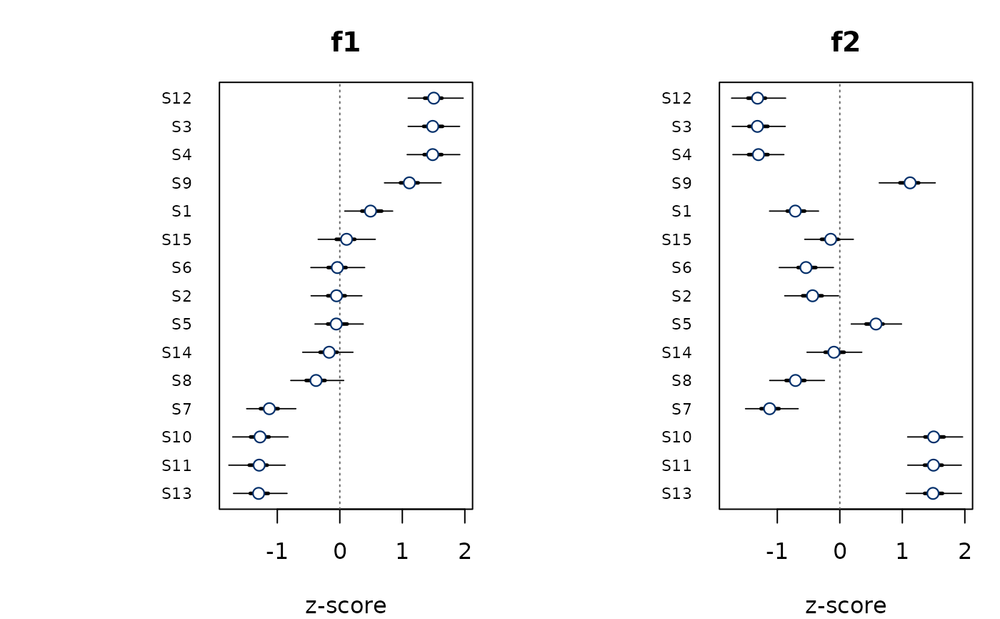
fit <- demo_fit(N = 12, J = 15, K = 2)
plot(fit)

summary(fit)
#> Bayesian Q-methodology factor model
#>   Call:      fit_bayesian(Y, K = K)
#>   Family:    Student-t (nu = estimated)
#>   Factors:   K = 2
#>   Data:      N = 12 persons, J = 15 statements
#>   Draws:     4 chains x 1000 post-warmup = 4000 total
#>   Backend:   demo
#>   Fitted:    2026-06-10 02:19:15
#>   Max Rhat:  1.010
#>   Min ESS:   bulk 820 / tail 950
#>   Divergent: 0
#> 
#> Factor characteristics:
#>    nload eigenvals expl_var
#> f1     6     3.204    26.70
#> f2     6     3.122    26.01
#> 
#> Hyperparameters (posterior summary):
#>  parameter   mean median     sd  lower  upper
#>         nu 20.233 20.246 4.2205 12.144 28.767
#>      sigma  0.498  0.500 0.0786  0.345  0.646
#>        tau  0.507  0.511 0.0820  0.358  0.660
#> 
#> Divergence summary:
#>   posterior median D_j ranges 0.20 to 2.81
#>   delta = 0.55 (reliability-adjusted critical difference)
#>   statements with P(D_j > delta | Y) >= 0.95: 7 of 15
#>   strongest consensus, max P(D_j < delta | Y): 0.94
#>   negative exemplars, P(dominant loading > 0 | Y) < 0.5: 0 of 12
#> 
#> MatchAlign diagnostics (mean Tucker phi per factor):
#>   f1 = 0.943  f2 = 0.945