This vignette walks through one Q study end to end in bayesqm: import, fit, diagnose, interpret, select K, and export. The running example is a synthetic 33-participant, 42-statement Q-sort.
Setup
bayesqm performs inference with Stan, so you need a working Stan backend before the modelling functions will run. The package supports cmdstanr (recommended) and rstan.
cmdstanr is distributed through the Stan R-universe rather than CRAN, and installing the R package does not install CmdStan itself; that is a separate step. Run the following once (not evaluated here):
install.packages("cmdstanr", repos = c("https://stan-dev.r-universe.dev", getOption("repos")))
cmdstanr::check_cmdstan_toolchain(fix = TRUE)
cmdstanr::install_cmdstan()
cmdstanr::cmdstan_version()   # should print a version
On Windows you additionally need Rtools matching your R version; on
macOS, run xcode-select --install. If you prefer rstan,
install it from CRAN with a C++ toolchain; bayesqm uses whichever
backend is available.
The remainder of this vignette uses small precomputed demonstration
objects (demo_fit(), demo_run()) so it renders
without a Stan backend. To reproduce the examples on real data you will
need the backend installed as above.
The Q-sort data
A Q study asks each participant to rank-order a set of statements
into a forced distribution. bayesqm represents that as a
J × N numeric matrix (statements as rows, participants as
columns) plus a vector of forced-distribution counts.
read_qsort() auto-detects the file format:
qdata <- read_qsort("mystudy.csv")   # CSV / Excel / HTMLQ / FlashQ
qdata <- read_qsort("mystudy.DAT")   # PQMethod
qdata <- read_qsort("mystudy.zip")   # KADE project
The example dataset:
sim   <- generate_data(N = 33, J = 42, K = 3, seed = 1)
qdata <- qsort_data(sim$Y, distribution = sim$distribution)
qdata
#> Q-sort data
#>   statements  : 42   participants : 33
#>   distribution: 2 3 4 5 7 7 5 4 3 2   (sum = 42 )
#>   value range : [-5, 5]
#>   source      : manual
Fitting the model
fit_bayesian() samples the posterior of a low-rank
factor model with a Student-t likelihood (by default) and a hierarchical
normal prior on the loadings, then resolves rotational ambiguity with
the MatchAlign post-processing of Poworoznek et
al. (2025):
fit <- fit_bayesian(qdata, K = 3, chains = 4, iter = 2000,
                    warmup = 1000, seed = 1)
fit <- demo_fit(N = 33, J = 42, K = 3, seed = 1)
fit
#> Bayesian Q-methodology factor model
#> Call: fit_bayesian(Y, K = K)
#> Family: Student-t (nu = estimated)
#> Factors: K = 3
#> Data: N = 33 persons, J = 42 statements
#> Draws: 4 chains x 1000 post-warmup = 4000 total
#> Backend: demo
#> Fitted: 2026-06-10 02:19:22
#> Max Rhat: 1.010
#> Min ESS: bulk 820 / tail 950
#> Divergent: 0
#>
#> Factor loadings (posterior median [95% CI], first 10 of 33 persons):
#> f1 f2 f3
#> P1 0.82 [0.66, 0.97] -0.04 [-0.21, 0.12] 0.02 [-0.15, 0.19]
#> P2 -0.09 [-0.24, 0.07] 0.74 [0.58, 0.91] 0.13 [-0.03, 0.29]
#> P3 0.04 [-0.13, 0.19] -0.12 [-0.30, 0.04] 0.60 [0.44, 0.77]
#> P4 0.69 [0.53, 0.86] -0.03 [-0.20, 0.12] 0.08 [-0.06, 0.24]
#> P5 0.06 [-0.08, 0.21] 0.78 [0.63, 0.94] -0.04 [-0.19, 0.11]
#> P6 0.13 [-0.02, 0.32] -0.08 [-0.26, 0.08] 0.59 [0.42, 0.71]
#> P7 0.67 [0.50, 0.82] -0.04 [-0.19, 0.13] -0.15 [-0.32, 0.01]
#> P8 0.11 [-0.03, 0.25] 0.74 [0.59, 0.89] -0.00 [-0.16, 0.15]
#> P9 -0.01 [-0.15, 0.12] -0.10 [-0.25, 0.04] 0.75 [0.60, 0.90]
#> P10 0.68 [0.51, 0.83] -0.12 [-0.27, 0.04] 0.06 [-0.08, 0.22]
#> ... (23 more; see fit$loa_median / fit$ci_lower / fit$ci_upper)
#>
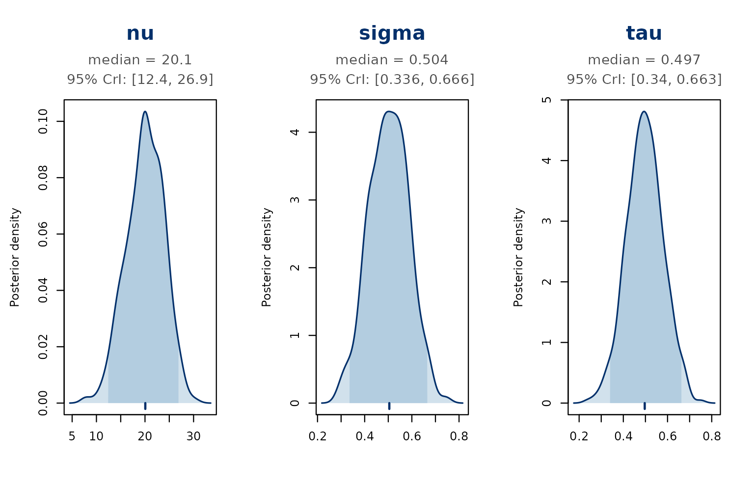
#> Hyperparameters:
#> parameter mean median sd lower upper
#> nu 20.0 20.1 3.818 12.41 26.89
#> sigma 0.5 0.5 0.083 0.34 0.67
#> tau 0.5 0.5 0.082 0.34 0.66
#>
#> Use summary() for factor characteristics, the divergence summary, and LOO.summary(fit) adds factor characteristics, the PSIS-LOO
ELPD (when available), a divergence summary, and the MatchAlign
diagnostic.
Diagnostics
Convergence statistics are stored on fit$diagnostics.
The recommended thresholds are R-hat below 1.01, bulk and tail effective
sample sizes above 400, and zero divergent transitions (Vehtari et al.
2021):
fit$diagnostics
#> $rhat_max
#> [1] 1.01
#>
#> $ess_bulk
#> [1] 820
#>
#> $ess_tail
#> [1] 950
#>
#> $divergences
#> [1] 0
plot_tucker() visualises the per-draw Tucker phi between
each aligned factor column and the MatchAlign pivot. Values near 1
indicate a stable alignment; bimodality signals residual
label-switching.
plot_tucker(fit)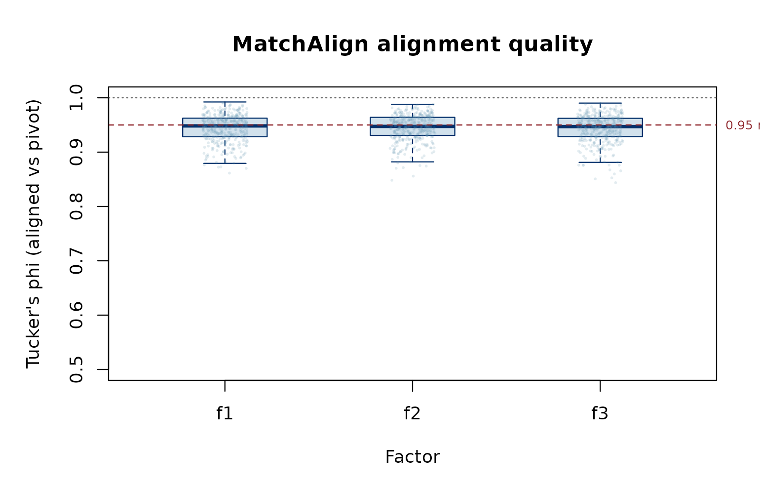
MatchAlign alignment quality by factor.
Factor loadings
Each participant has a posterior distribution over their loading on
every factor. plot_loading_posterior() draws the loading
forest, with nested 50% and 95% credible-interval whiskers and the
classical Brown (1980) cut-off as a faint reference.
Filled points are participants with
P(factor k dominant) > 0.5.
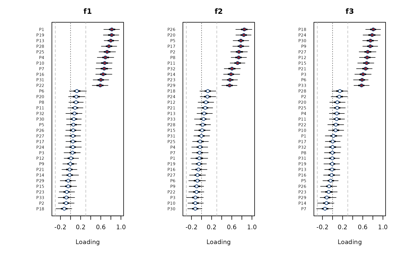
Loadings with nested 50% and 95% credible intervals.
The same information as a tidy data frame:
head(compute_loadings(fit$Lambda_draws, prob = 0.95))
#>   participant      f1_loa    f1_lower   f1_upper      f2_loa   f2_lower
#> 1          P1  0.82218583  0.65967029 0.97347665 -0.04267266 -0.2145922
#> 2          P2 -0.08886156 -0.24309784 0.07209832  0.74522036  0.5791526
#> 3          P3  0.03940137 -0.12972350 0.19405389 -0.12287342 -0.2986770
#> 4          P4  0.69365900  0.53025182 0.85839822 -0.03571152 -0.1965369
#> 5          P5  0.05989579 -0.07856949 0.21054518  0.78202658  0.6258714
#> 6          P6  0.12982142 -0.02363006 0.31509987 -0.08730420 -0.2556340
#>     f2_upper      f3_loa    f3_lower  f3_upper
#> 1 0.12335192  0.01982447 -0.14521623 0.1878235
#> 2 0.91064671  0.13579980 -0.02821464 0.2948461
#> 3 0.03507329  0.60443673  0.44105818 0.7671924
#> 4 0.12328690  0.08182326 -0.06409235 0.2354870
#> 5 0.93757307 -0.03495072 -0.19214191 0.1134495
#> 6 0.07939546  0.58198954  0.41551318 0.7077884
Factor z-scores
plot() produces a cross-panel z-score dotchart; rows
share an order (by factor 1’s posterior mean, configurable via
sort_by) so factors can be compared horizontally.
plot(fit)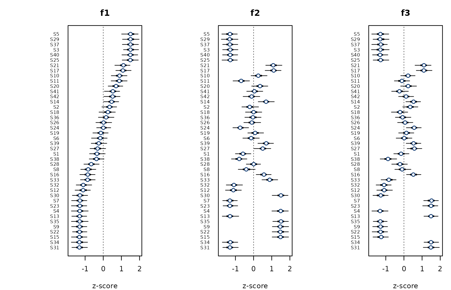
Posterior z-scores across factors with 50% and 95% credible intervals.
For a single statement across factors,
plot_zscore_posterior() shows the per-factor view:
plot_zscore_posterior(fit, statement = 1)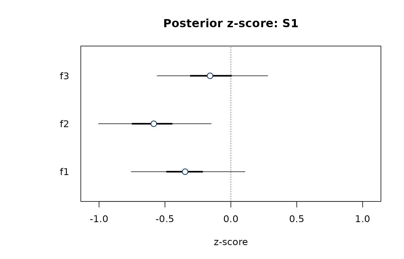
Posterior z-score for a single statement across factors.
Choosing K
run_bayes() fits the model for each K in a range and
applies the peak-plus-Sivula protocol: the ELPD peak is
the automated choice and the Sivula parsimony rule (Sivula et al.
2025) is reported alongside as a diagnostic.
On real data:
run <- run_bayes(qdata, K_max = 4, seed = 1,
                 chains = 2, iter = 1500, warmup = 800)
run <- demo_run(K_max = 5, k_peak = 3, k_sivula = 1, case = "gap")
run
#> Bayesian Q-methodology: multi-K comparison
#>   K range:      1..5
#>   ELPD peak:    K = 3  (automated adoption)
#>   Sivula rule:  K = 1  (parsimony diagnostic)
#>   Case:         gap  (ELPD peak > Sivula (weak discrimination between adjacent models))
#>
#> LOO comparison:
#>  K    elpd   se delta_elpd se_delta ratio
#>  1 -180.09 8.00
#>  2 -170.91 7.25      -9.18     3.00  3.06
#>  3 -165.42 6.50      -5.49     3.00  1.83
#>  4 -170.20 5.75       4.78     3.00  1.59
#>  5 -179.61 5.00       9.41     3.00  3.14
#>
#> Case 'gap': k_peak is adopted; Sivula is reported as a parsimony diagnostic only.
make_elpd_diff(run)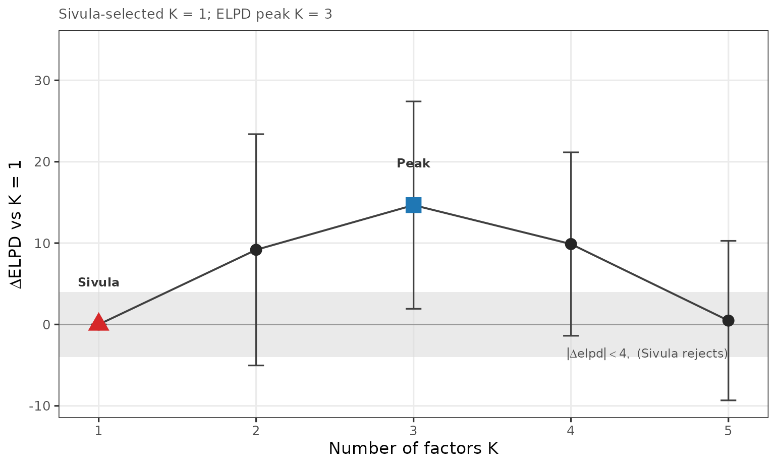
ΔELPD across K with the Sivula non-promotion band at |ΔELPD| < 4. Triangle marks the Sivula K, square marks the ELPD peak (the adopted K).
The ELPD peak is always the adopted K. The Sivula diagnostic is
reported alongside as a parsimony check. The run$case field
labels the relationship between the two: when Sivula lands on the same K
as the peak, the case is agree; when Sivula points to a
smaller K than the peak, the case is gap; when Sivula
exceeds the peak, the case is reversed (rare in
practice).
Distinguishing, consensus, and membership
bayesqm replaces the classical z-score test with the
posterior of an explicit viewpoint-divergence measure. For each
statement, D_j is the mean absolute pairwise difference of the K
viewpoint scores; the package reports P(D_j > delta | Y) and P(D_j
< delta | Y), the probabilities that the viewpoints diverge
meaningfully or practically agree. By default the separation delta is
the reliability-adjusted critical difference from classical Q analysis
(Brown 1980),
computed from the posterior dominant-factor counts
(critical_delta()); suggest_delta() (one
forced-distribution category on the standardised scale) is an
alternative, and results are reported with sensitivity across the choice
of delta. No fixed probability cutoff defines a statement.
The full distinguishing/consensus table is stored on
fit$qdc (per viewpoint: grid position and z-score with 95%
CrI, then D_j with 95% CrI, pi_D,
pi_C). critical_delta() returns the separation
the fit used:
critical_delta(fit$Lambda_draws)
#> [1] 0.4131967
head(fit$qdc)
#>   statement f1_grid     f1_zsc    f1_lower   f1_upper f2_grid     f2_zsc
#> 1        S1      -1 -0.3436199 -0.75598677  0.1066338      -1 -0.5924826
#> 2        S2       1  0.3356155 -0.07696179  0.7385355      -1 -0.2080451
#> 3        S3       4  1.4979823  1.11477391  1.9446729      -3 -1.2921554
#> 4        S4      -2 -1.2847601 -1.75639810 -0.8298201       4  1.4848346
#> 5        S5       5  1.5174761  1.01119678  1.9237407      -5 -1.3155732
#> 6        S6       1 -0.1660726 -0.64869137  0.2149788      -1 -0.1410127
#>     f2_lower   f2_upper f3_grid      f3_zsc    f3_lower   f3_upper  D_median
#> 1 -1.0039154 -0.1486896      -1 -0.15075033 -0.55964521  0.2793994 0.3381550
#> 2 -0.6461072  0.2744403       2  0.34784928 -0.06702773  0.7702793 0.4427912
#> 3 -1.7067359 -0.8610203      -3 -1.29522175 -1.79044451 -0.8143189 1.9525495
#> 4  1.0077216  1.9142497      -5 -1.30747085 -1.76660521 -0.8738692 1.9386399
#> 5 -1.7515059 -0.8978920      -4 -1.30529856 -1.77439164 -0.8363799 1.9742330
#> 6 -0.5929771  0.3163001       1  0.01668352 -0.42748367  0.4427847 0.2651122
#>      D_lower   D_upper   pi_D   pi_C
#> 1 0.06190555 0.7146339 0.3725 0.6275
#> 2 0.13551050 0.8479464 0.5825 0.4175
#> 3 1.58449898 2.2832984 1.0000 0.0000
#> 4 1.55679839 2.3175306 1.0000 0.0000
#> 5 1.54433252 2.3631369 1.0000 0.0000
#> 6 0.04975712 0.6005598 0.1900 0.8100
plot_dist_cons(fit)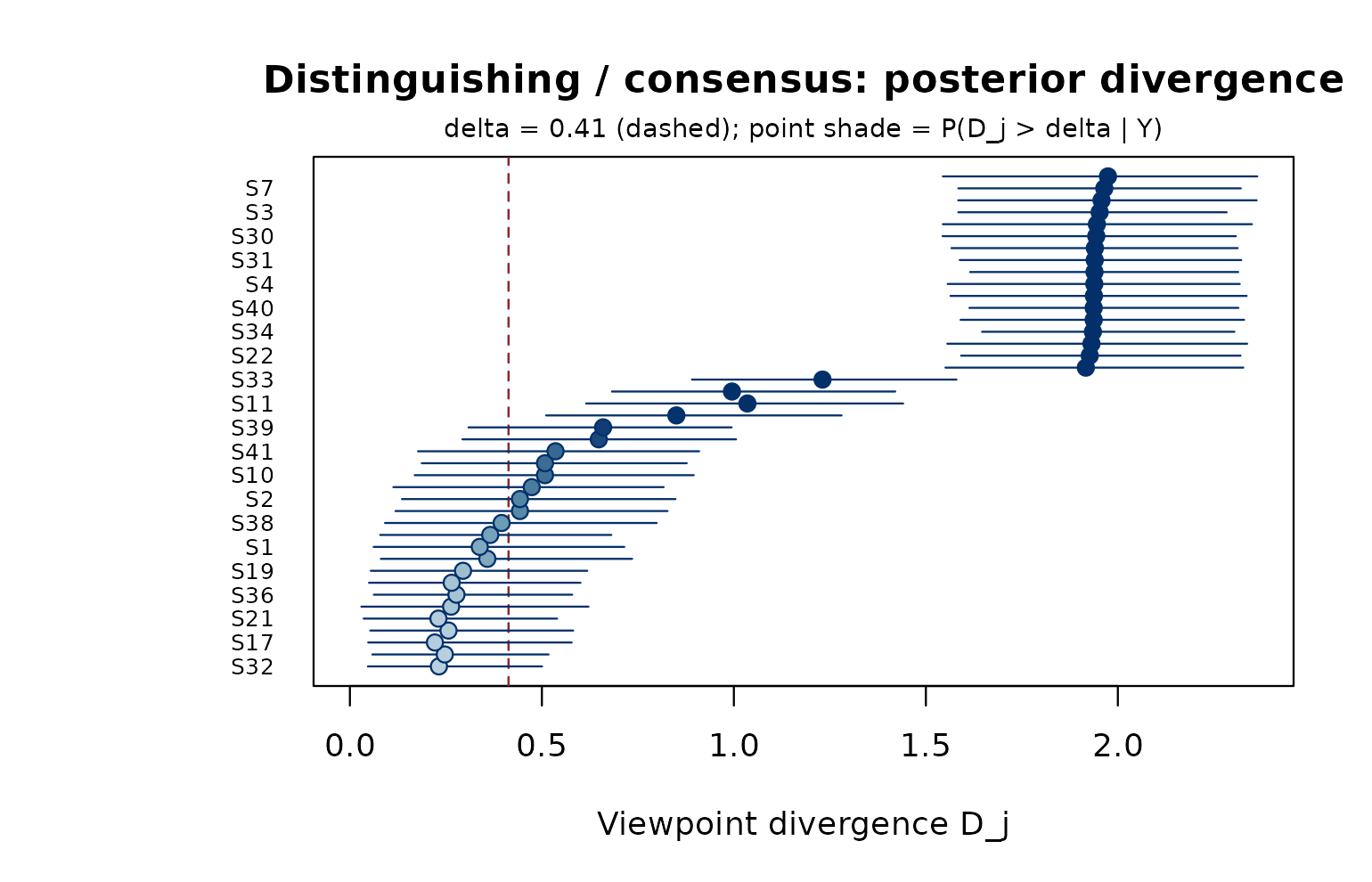
Posterior viewpoint divergence D_j with 95% credible intervals; statements ordered by P(D_j > delta | Y).
Participant-level membership is also probabilistic.
classify_membership() turns posterior dominance into a
Strong / Moderate / Weak tier:
head(classify_membership(fit$Lambda_draws))
#>   participant dominant_factor dominant_label max_prob   tier
#> 1          P1               1             f1        1 Strong
#> 2          P2               2             f2        1 Strong
#> 3          P3               3             f3        1 Strong
#> 4          P4               1             f1        1 Strong
#> 5          P5               2             f2        1 Strong
#> 6          P6               3             f3        1 Strong
make_dominant_panel(fit)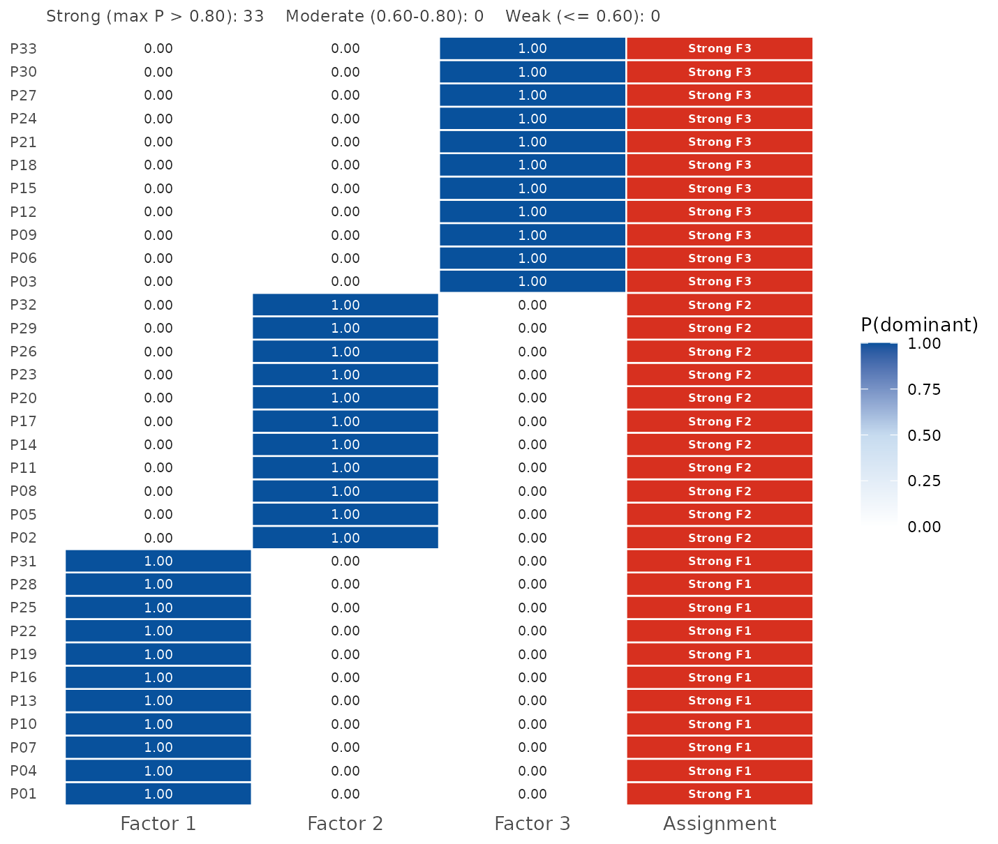
Blue tiles: posterior probability that each factor is dominant for a given participant (values printed in each cell). The right column shows the overall assignment verdict on an orange-red scale.
Posterior predictive check
plot_ppc() shows the posterior distribution of the RMSE
between cor(Y_rep) and cor(Y_obs). A
well-specified model puts most posterior mass at small RMSE.
plot_ppc(fit)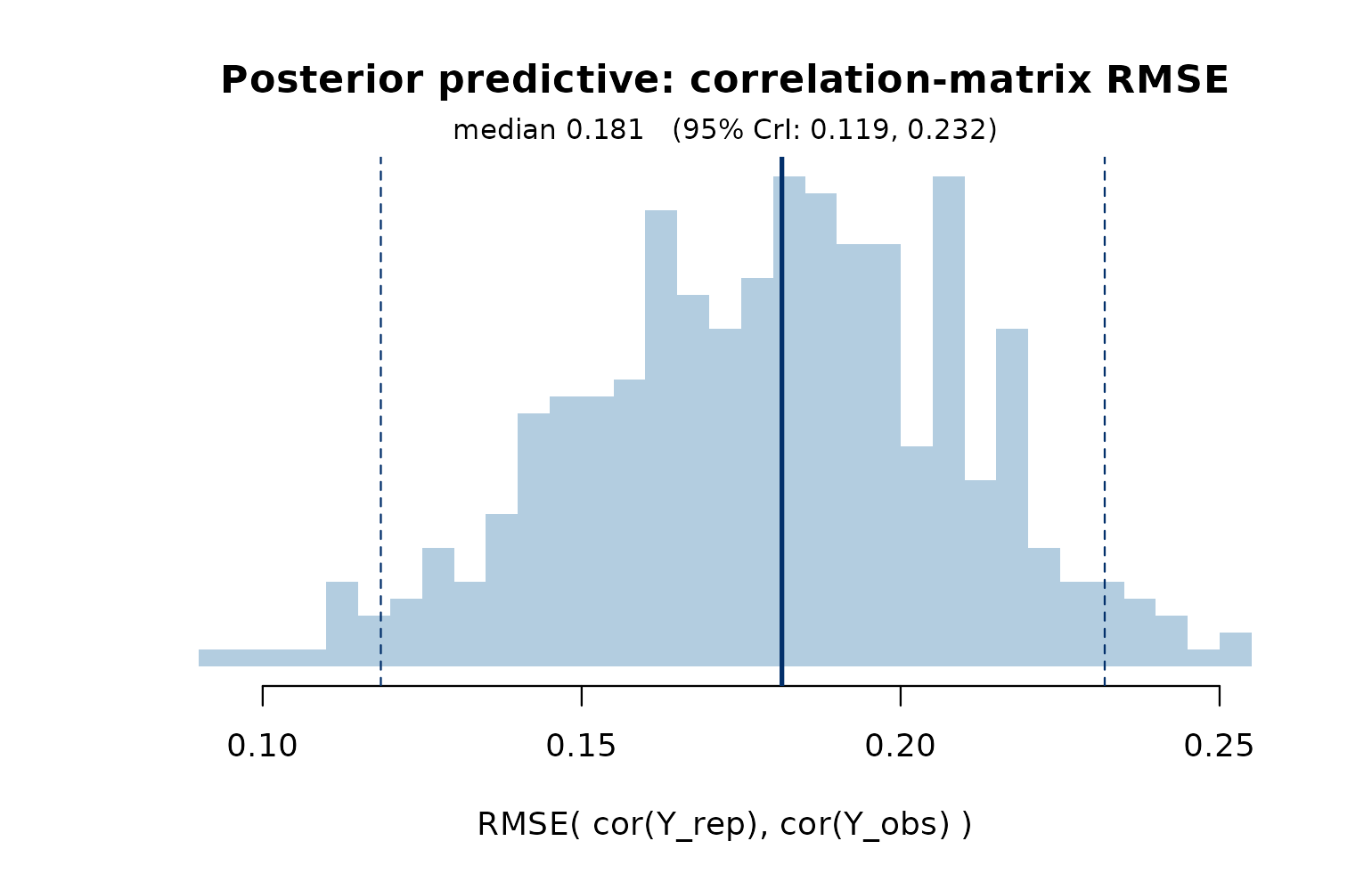
PPC on the by-person correlation matrix.
Reporting and exporting
save_bayesqm_plot() writes any plot to PDF, SVG, PNG,
TIFF, or JPEG at the chosen dimensions:
save_bayesqm_plot("fig_loadings.pdf", plot_loading_posterior(fit))
save_bayesqm_plot("fig_elpd.pdf",      plot_elpd(run),
                  width = 3.5, height = 3)
caption_bayesqm() returns a figure caption with model
configuration, sample sizes, interval probability, and convergence
diagnostics:
caption_bayesqm(fit)
#> [1] "Bayesian Q-methodology factor model (K = 3, N = 33, J = 42); fitted with a Student-t likelihood via demo (4 chains, 4,000 post-warmup draws); intervals shown at 95% posterior coverage; max Rhat = 1.010, min bulk ESS = 820, 0 divergent transitions. Fitted with the bayesqm R package."
Standard R accessors work on the fit (coef,
fitted, residuals, sigma,
family, as.matrix), and
as.matrix(fit) returns a Stan-style draws matrix that
posterior and bayesplot consume natively.
Theming
Every plot reads its palette through bayesqm_colors().
Switch the scheme once and every subsequent base-R plot follows:
bayesqm_set_colors("teal")   # "blue" (default), "red", "purple", "grey"
plot(fit)
bayesqm_set_colors("blue")
Where next
-
?fit_bayesian: every prior and sampler option -
?run_bayes: peak-plus-Sivula thresholds -
?bayesqm-membership: the full set of membership summaries -
?rename_factors: relabelf1..fKwith substantive factor names -
ggplot2::autoplot(): ggplot2 / ggdist versions of every view above, whenggplot2andggdistare installed