
The idea, and a rule to remember
Every other article runs one method on one recording. A study runs
every method on every recording, and then has to put the numbers
somewhere a collaborator can open. That is what this family is for:
circadian.batch() runs the whole analysis over a folder of
.agd files and returns one tidy row per
file; circadian.workbook() writes the complete
analysis of a single recording to a multi-sheet Excel file; and
circadian.daily() breaks a recording into per-day rows so
within-recording drift shows instead of being averaged away. Above the
single subject, population.cosinor() and
cosinor.compare() pool per-subject fits into a group rhythm
and test whether two groups differ.
The rule to carry through this article: one row per file, and
a bad file costs you a cell, not the run.
circadian.batch() wraps each file in its own error handler,
so a recording that fails to read or analyse lands in an
error column with NA metrics while every other
file completes. A batch that aborts on file 37 of 200 is worse than
useless; a batch that flags file 37 and finishes is a study you can act
on.
The shape of a run
There is no equation here (the family is plumbing, not a model), but the output has a fixed shape worth stating up front.
-
circadian.batch()returns a data frame: afilecolumn, anerrorcolumn, and then the full single-row summary thatcircadian.workbook()builds internally (the nonparametric IS/IV/RA/L5/M10, the cosinor MESOR/amplitude/acrophase and its rhythmicity F-test, the Lomb-Scargle and chi-square periods, DFA and multifractal width, multiscale entropy, and the rest-activity transition rates). Every file is one row; every metric is one column. -
circadian.workbook()writes that same summary as the first sheet of an.xlsx, then adds detail sheets (the hourly profile, both periodograms, the fluctuation and multifractal spectra, the transition curves) and a self-documenting Data Dictionary sheet, the same single source the output codebook renders from. -
circadian.daily()returns adailydata frame with one row per calendar day (L5,M10, their onset hours,RA,IV, and the day’s total counts).
Knowing the shape is most of knowing how to script against it.
Assumptions, and when they break
-
Readable, regularly-epoched files. The batch
assumes each path is an
.agdActiGraph fileread.agd()can open. Anything else becomes anerrorrow, which is the design, not a failure. -
A consistent epoch across files. By default the
epoch is inferred per file from the timestamps; mixing 30 s and 60 s
recordings is allowed, but the epoch-sensitive metrics (IV especially)
are then only comparable within an epoch. Pass an explicit
epoch_lengthto force one. -
Enough valid days per file. The per-day and
between-day metrics need whole days;
circadian.daily()drops any day with fewer thanmin_hoursof valid recording before reporting it. -
Subjects, not epochs, are the unit for the group
tools.
population.cosinor()andcosinor.compare()fit one cosinor per subject and then pool; they assume each subject contributes an averaged 24-hour profile with at leastmin_valid_hoursof data. They are not a substitute for a mixed model. See Choosing a method for when to reach for one.
Recovering known truth
Before trusting the group tools on real cohorts, watch them recover a difference we plant. We build two groups of six subjects each: a morning group whose rhythm peaks at 08:00 with amplitude 45, and an evening group peaking at 13:00 with amplitude 38. Both share a MESOR of 100. The planted between-group acrophase difference is exactly five hours.
set.seed(42)
hrs <- 0:23
act <- ts <- subj <- grp <- NULL
for (g in c("morning", "evening")) for (i in 1:6) {
  acro <- if (g == "morning") 8 else 13
  amp  <- if (g == "morning") 45 else 38
  y <- 100 + amp * cos(2 * pi * (hrs - acro) / 24) + rnorm(24, 0, 5)
  act  <- c(act, y)
  subj <- c(subj, rep(paste0(substr(g, 1, 1), i), 24))
  grp  <- c(grp, rep(g, 24))
  ts   <- c(ts, as.POSIXct("2024-01-01", tz = "UTC") + hrs * 3600)
}
ts <- as.POSIXct(ts, tz = "UTC", origin = "1970-01-01")
population.cosinor() pools each group’s per-subject fits
into a Bingham group-mean rhythm with confidence intervals (Bingham et al.,
1982). It should return the planted MESOR, amplitude, and
acrophase for each group.
pc <- population.cosinor(act, ts, subject = subj, group = grp)
knitr::kable(
  data.frame(
    group     = c("morning", "evening"),
    planted_acrophase = c(8, 13),
    recovered_acrophase = c(pc$morning$acrophase, pc$evening$acrophase),
    planted_amplitude = c(45, 38),
    recovered_amplitude = c(pc$morning$amplitude, pc$evening$amplitude)
  ),
  digits = 2,
  caption = "The population cosinor recovers each group's planted acrophase and amplitude."
)| group | planted_acrophase | recovered_acrophase | planted_amplitude | recovered_amplitude |
|---|---|---|---|---|
| morning | 8 | 8.48 | 45 | 45.41 |
| evening | 13 | 13.49 | 38 | 37.38 |
cosinor.compare() then tests whether the two groups
differ. The amplitude/acrophase test is a two-variate Hotelling
on the (cosine, sine) coefficients (Bingham et al., 1982); the MESOR
difference is a separate pooled-variance F-test. The per-parameter rows
break both down, with the acrophase test made circular-aware.
cmp <- cosinor.compare(act, ts, subject = subj, group = grp)
cmp
#> Cosinor Comparison Between Two Groups
#>
#>   Groups:  evening (n=6)  vs  morning (n=6)
#>   Period:  24 h
#>
#>   Amplitude/acrophase (Bingham T2):  F(2,9) = 966.39   p = 3.14e-11
#>   MESOR (Bingham F):                 F(1,10) = 0.05   p = 0.82
#>
#>   mesor     diff = +0.11   t(7.5) = 0.23   p = 0.821
#>   amplitude diff = -8.04   t(7.3) = -9.27   p = 2.62e-05
#>   acrophase diff = +5.00   t(9.1) = 61.49   p = 3.3e-13
The omnibus is overwhelmingly significant, and the per-parameter breakdown lands where we planted it: the MESOR difference is near zero, the amplitude differs by about the planted seven units, and the acrophase difference recovers the planted five hours. The tools report exactly the contrast we put in.
On a real recording
The bundled extdata folder holds the package’s example
.agd files. Pointing circadian.batch() at the
directory analyses every file in it and returns one row each.
folder <- system.file("extdata", package = "actiRhythm")
batch  <- circadian.batch(folder, verbose = FALSE)
nrow(batch)
#> [1] 2
batch[, c("file", "error", "IS", "IV", "RA",
          "cosinor_amplitude", "rhythm_p_value", "period_tau")]
#>                      file error     IS     IV     RA cosinor_amplitude
#> 1 MOS2E39230594_60sec.agd  <NA> 0.2279 1.0008 0.9800            295.63
#> 2  MOS2E3923063660sec.agd  <NA> 0.4230 1.2687 0.7706            351.14
#>   rhythm_p_value period_tau
#> 1    0.002396228   24.89529
#> 2    0.050151893   24.08320
Two files in, two rows out, with error all
NA (both read and analysed cleanly), and the full metric
set sitting alongside in columns we have only sampled here. Each row
carries everything the output
codebook documents.
To see within a recording rather than across files,
circadian.daily() reports each calendar day on its own.
agd   <- agd.counts(read.agd(example_agd(1), verbose = FALSE))
daily <- circadian.daily(agd$axis1, agd$timestamp)
daily
#> Per-Day Nonparametric Metrics (7 days)
#>
#>        date     L5 L5_onset_h      M10 M10_onset_h    RA    IV   total
#>  2025-10-08  8.590      0.200 1190.400      10.533 0.986 1.342  961265
#>  2025-10-09 12.883      1.900 1038.933      13.667 0.976 1.032  804120
#>  2025-10-10 15.660      1.433 1657.895      12.050 0.981 1.628 1247818
#>  2025-10-11  0.000      1.833    0.445      15.833 1.000 2.291     445
#>  2025-10-12  0.000      0.000    0.075      13.783 1.000 1.533      78
#>  2025-10-13  0.000      0.567    0.405      22.550 1.000 0.988     243
#>  2025-10-14  0.000      0.000   14.171      14.000 1.000 1.121    6313
ggplot(daily$daily, aes(date, M10_onset_h)) +
  geom_line(colour = "grey60") +
  geom_point(colour = "#236192", size = 2) +
  labs(x = NULL, y = "M10 onset (h)") +
  theme_actiRhythm()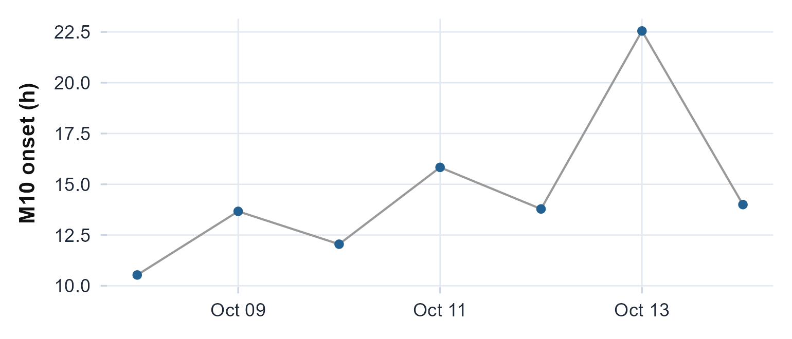
The most-active-window onset for each day. Reporting it per day, rather than pooled into the batch row, shows how steady the active phase is across the recording.
Reading the numbers
The batch row is only as useful as your sense of what each column should be. A few human yardsticks for scanning a study-sized table:
-
erroris the first column to read, not the last. Sort or filter on it before trusting any metric; a non-NAvalue means that row’s numbers are missing, not that the subject has a flat rhythm. -
rhythm_p_valuebelow 0.05 says the day-night cosine is real, but read it withpercent_rhythm(how much of the day the single cosine captures) andIS/IV(how stable and how fragmented), exactly as in the cosinor and nonparametric articles. The batch just lines those columns up side by side. -
period_taunear 24 is an entrained rhythm; a value drifting from 24 across a cohort is the cue to look at free-running, not a rounding error. - For the group comparison, an omnibus p-value answers “do the rhythms differ at all?” before you read any single parameter; the per-parameter rows then say which parameter carries the difference, with the acrophase row already unwrapped around the clock.
The wider reporting family
The same machinery feeds two output formats a collaborator can open directly.
A full single-subject workbook.
circadian.workbook() runs every method on one recording and
writes a multi-sheet .xlsx: the one-row summary, a detail
sheet per analysis, and a Data Dictionary. Here we write it to a
temporary file and list its sheets. (The chunk is guarded so it only
runs where openxlsx is installed.)
xlsx <- tempfile(fileext = ".xlsx")
circadian.workbook(agd$axis1, agd$timestamp, file = xlsx, include_period_ci = FALSE)
openxlsx::getSheetNames(xlsx)
#>  [1] "Summary"                  "Hourly Profile"
#>  [3] "Lomb-Scargle Periodogram" "Chi-square Periodogram"
#>  [5] "Fractal DFA"              "MF-DFA"
#>  [7] "Multiscale Entropy"       "Rest-Active Transitions"
#>  [9] "Active-Rest Transitions"  "Data Dictionary"
circadian.batch() accepts the same file =
argument to write a single workbook whose Summary sheet has one row per
file, the study-level companion to the per-subject workbook above.
Saving a figure. save.circadian.plot()
is a thin wrapper over ggplot2::ggsave() that takes any of
the package’s plot_* figures and writes it in the format
implied by the file extension, so a report script can emit its actograms
without restating the size and DPI each time.
p   <- plot_actogram(agd$axis1, agd$timestamp)
png <- tempfile(fileext = ".png")
save.circadian.plot(p, png, width = 8, height = 5)
file.exists(png)
#> [1] TRUE
Limitations
-
Speed scales with the slowest method, times the number of
files. The bootstrap period CI is off by default in
circadian.batch()(include_period_ci = FALSE) for exactly this reason; turn it on only when you need it. -
An
errorrow is a missing subject, not a fixed one. The batch keeps running, but you still have to go back and find out why a file failed to read. -
The group tools pool, they do not model.
population.cosinor()andcosinor.compare()average per-subject fits and run a two-sample test; they do not borrow strength across subjects or handle nested designs. For repeated measures or covariates, the mixed-model route in Choosing a method is the right tool. - Column meanings live in one place. Rather than memorise 40-plus column names, read them from the Data Dictionary sheet or the output codebook; both render from the same source file.
Reference and validation
The two group tools implement the population-mean cosinor and
between-group comparison of Bingham et al. (1982):
population.cosinor() averages the linearized per-subject
coefficients into a Bingham group rhythm with confidence intervals, and
cosinor.compare() runs the Bingham / Hotelling
omnibus alongside circular-aware per-parameter tests. Every metric a
batch row or workbook reports is the same quantity validated in its own
article (the cosinor and nonparametric families are cross-checked
against reference implementations in the Validation article), and the meaning of each
column is documented in the output
codebook.