
This article continues from the get-started vignette and works from raw accelerometer data rather than activity counts. It shows how actiRhythm reads raw ActiGraph, Axivity, and GENEActiv files, auto-calibrates them, derives the ENMO, MAD, and z-angle metrics, runs the full circadian analysis and a posture-based sleep detector directly from a file, and checks both the per-epoch metrics and the sleep window against GGIR. The objects below are rebuilt here so the article stands on its own.
agd <- agd.counts(read.agd(example_agd(1), verbose = FALSE))
raw <- example_raw(days = 2)        # synthetic 2-day recording (or a real file path)

# Real .gt3x used only for the GGIR cross-check at the end. It lives in data-raw/
# (kept in the source repo, excluded from the CRAN build), so the cross-check runs
# when the repo is present and is skipped otherwise.
gt3x_file <- local({
  cands <- c("../../data-raw/MOS2E39230594.gt3x", "data-raw/MOS2E39230594.gt3x")
  inp <- tryCatch(knitr::current_input(dir = TRUE), error = function(e) NULL)
  if (!is.null(inp))
    cands <- c(file.path(dirname(inp), "..", "..", "data-raw", "MOS2E39230594.gt3x"), cands)
  root  <- tryCatch(rprojroot::find_root(rprojroot::has_file("DESCRIPTION")),
                    error = function(e) NULL)
  if (!is.null(root)) cands <- c(cands, file.path(root, "data-raw", "MOS2E39230594.gt3x"))
  hit <- cands[file.exists(cands)]
  if (length(hit)) normalizePath(hit[1]) else NA_character_
})
Raw metrics and posture
Everything so far runs on activity counts. Raw accelerometer files
also record the gravity component, and with it body posture, which
counts cannot carry. actiRhythm reads the three common formats:
ActiGraph .gt3x, Axivity .cwa, and GENEActiv
.bin.
raw.metrics() takes a file path. Raw acceleration is far
too large to bundle, so for a reproducible illustration
example_raw() synthesises a recording; a real file is read
the same way, with raw.metrics("recording.cwa").
m <- raw.metrics(raw, epoch = 60)   # per-epoch ENMO (mg), MAD, and the z-angle
head(m)
#>                  time     ENMO      MAD    anglez
#> 1 2024-01-01 12:00:00 43.95883 24.78791  8.280445
#> 2 2024-01-01 12:01:00 43.13860 24.89003 14.666095
#> 3 2024-01-01 12:02:00 44.56626 25.55921  8.287697
#> 4 2024-01-01 12:03:00 44.25995 24.90778 14.705513
#> 5 2024-01-01 12:04:00 44.79032 25.36485  8.292428
#> 6 2024-01-01 12:05:00 44.17071 24.72920 14.755796
plot_raw_metrics(raw, epoch_length = 60)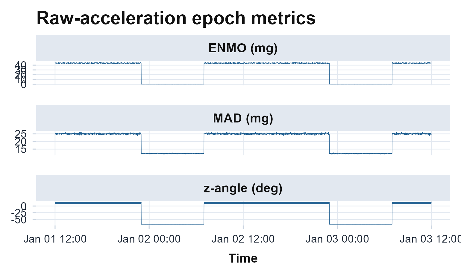
The three raw-acceleration epoch metrics across the recording: ENMO and MAD (movement, in mg) are low at night, while the z-angle (degrees) tracks arm posture.
ENMO is the activity signal, and every method above takes it
directly: pass it to circadian.rhythm(), or let
circadian.raw() run the whole analysis from the file.
cr <- circadian.rhythm(m$ENMO, m$time)
c(IS = cr$IS, IV = cr$IV, RA = cr$RA)
#>     IS     IV     RA
#> 1.0000 0.3823 0.9873
Calibration is applied first inside raw.metrics().
auto.calibrate() finds the per-axis gain and offset that
return still periods to the 1 g sphere (Hees et al., 2014); on data with a
known distortion it returns the original gain and offset to within a
fraction of a percent.
set.seed(1)
u <- matrix(rnorm(40 * 3), 40, 3); u <- u / sqrt(rowSums(u^2))
cal <- do.call(rbind, lapply(seq_len(40), function(i)
  matrix(rep(u[i, ] / c(1.03, 0.97, 1.01) + c(0.04, -0.03, 0.02), each = 300),
         300, 3) + rnorm(900, 0, 0.004)))
auto.calibrate(data.frame(x = cal[, 1], y = cal[, 2], z = cal[, 3]),
               fs = 30)[c("scale", "offset")]
#> $scale
#> [1] 1.0301368 0.9701036 1.0099053
#>
#> $offset
#> [1]  0.04000830 -0.02992048  0.01990560
The z-angle supports a sleep detector that needs no diary and works
from posture, which the counts cannot do. rest.spt() finds
the nightly sleep-period-time window from the distribution of angle
change [HDCZA; Hees et al. (2018)], sib.vanhees()
scores sustained-inactivity bouts (Hees et al., 2015), and
sleep.from.spt() combines them into onset, wake and
efficiency. detect.nonwear.raw() flags a stationary,
taken-off device [low standard deviation and range over the hour; Hees et al. (2013)], and passing its mask as
wear keeps a device-off stretch from being read as one long
night. Computed here on the synthetic recording at a 5-second epoch,
with the detected windows shaded.
m5    <- raw.metrics(raw, epoch = 5, metrics = "anglez")
wear  <- detect.nonwear.raw(raw, epoch = 5)
spt   <- rest.spt(m5$anglez, m5$time, epoch_length = 5, wear = wear)
sib   <- sib.vanhees(m5$anglez, epoch_length = 5)
sleep <- sleep.from.spt(spt, sib, m5$time, epoch_length = 5)
plot_spt(raw)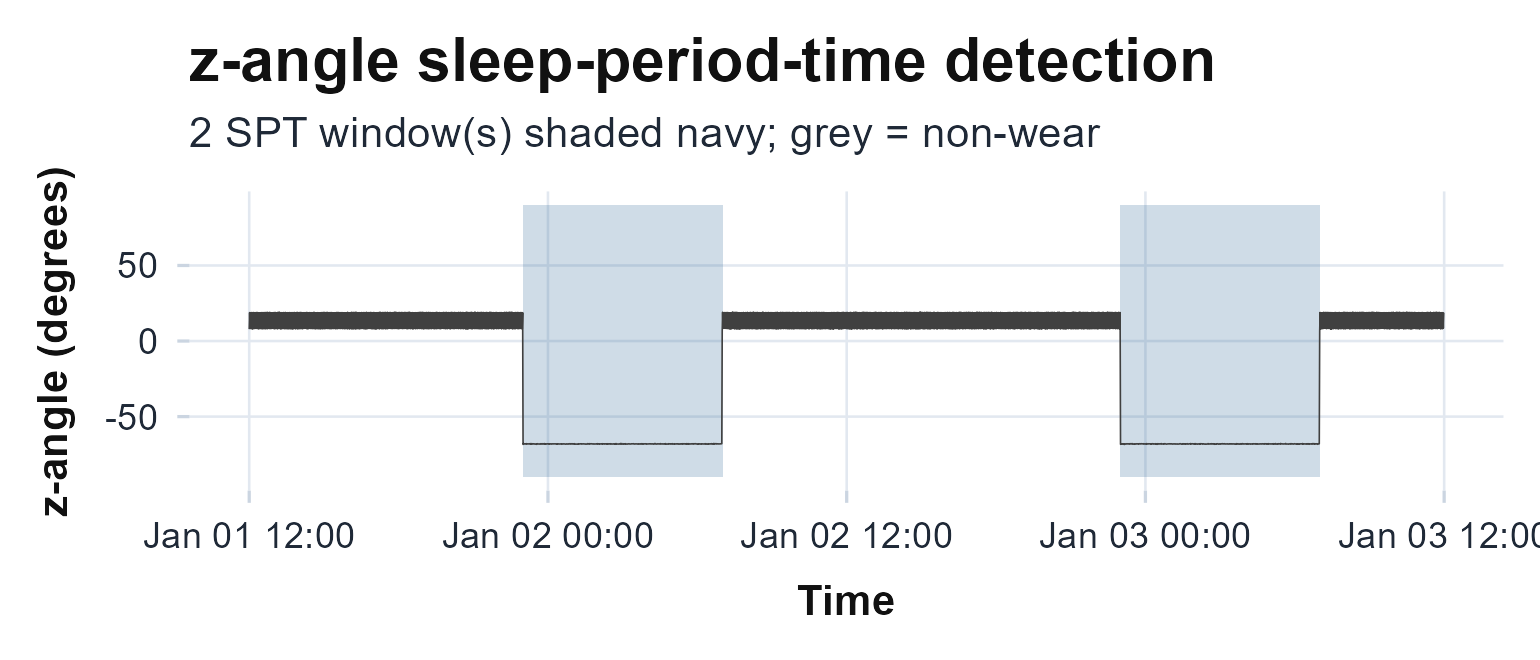
The z-angle of the synthetic recording at 5-second epochs, with the two nightly sleep-period-time windows shaded, each detected from the z-angle alone (HDCZA) and gated by raw non-wear.
sleep[, c("date", "onset", "offset", "tst", "efficiency")]
#>         date               onset              offset      tst efficiency
#> 1 2024-01-01 2024-01-01 23:00:00 2024-01-02 07:00:00 8.001389  0.9968853
#> 2 2024-01-02 2024-01-02 23:00:00 2024-01-03 07:00:00 8.001389  0.9968853
Two more estimators measure fragmentation, and both run on the counts
already loaded: activity.balance.index() maps a
detrended-fluctuation exponent to a 0 to 1 score that peaks at the
healthy 1/f balance (Danilevicz et al., 2024), and
transition.probability() gives the closed-form
rest-to-active and active-to-rest transition probabilities.
activity.balance.index(fractal.dfa(agd$axis1))
#> $ABI_overall
#> [1] 0.5803233
#>
#> $ABI_short
#> [1] 0.7336085
#>
#> $ABI_long
#> [1] 0.3710439
transition.probability(agd$axis1)[c("tp_ra_mle", "tp_ar_mle")]
#> $tp_ra_mle
#> [1] 0.04854369
#>
#> $tp_ar_mle
#> [1] 0.1366603
Agreement with GGIR
The raw metrics and the z-angle reimplement the van Hees algorithms
that GGIR established (Migueles et al., 2019), so they
should reproduce GGIR’s output, not merely be internally consistent. The
check below runs that comparison directly: it computes GGIR’s per-epoch
ENMO and z-angle (GGIR::g.getmeta()) and actiRhythm’s
(raw.metrics()) on the same real wrist recording and
measures how closely they agree.
That recording lives in the package’s data-raw/ folder
(kept in the source repository but excluded from the CRAN build, since a
multi-day raw file is far too large to ship), so the table is computed
whenever the repository and GGIR are present and skipped otherwise
(gt3x_file is resolved in the setup chunk).
P <- GGIR::load_params()
P$params_general$windowsizes <- c(5, 900, 3600)
I <- GGIR::g.inspectfile(gt3x_file, params_rawdata = P$params_rawdata,
                         params_general = P$params_general)
ggir <- GGIR::g.getmeta(gt3x_file, params_rawdata = P$params_rawdata,
                        params_general = P$params_general,
                        params_cleaning = P$params_cleaning,
                        inspectfileobject = I)$metashort
#>
#> Loading chunk: 1 2 3
acti <- raw.metrics(gt3x_file, epoch = 5)

# Align on the 5-second wall-clock label, then compare per epoch.
gg <- data.frame(k = gsub("T", " ", substr(as.character(ggir$timestamp), 1, 19)),
                 enmo = ggir$ENMO * 1000, anglez = ggir$anglez)
aa <- data.frame(k = format(acti$time, "%Y-%m-%d %H:%M:%S"),
                 enmo = acti$ENMO, anglez = acti$anglez)
m  <- merge(gg, aa, by = "k", suffixes = c("_ggir", "_acti"))

knitr::kable(
  data.frame(
    metric = c("ENMO (mg)", "z-angle (deg)"),
    cor    = c(cor(m$enmo_ggir, m$enmo_acti), cor(m$anglez_ggir, m$anglez_acti)),
    mad    = c(mean(abs(m$enmo_ggir - m$enmo_acti)),
               mean(abs(m$anglez_ggir - m$anglez_acti)))
  ),
  digits = c(0, 4, 2),
  col.names = c("Metric", "Correlation with GGIR", "Mean abs. difference"),
  caption = sprintf("Per-epoch agreement with GGIR over %s matched 5-second epochs.",
                    format(nrow(m), big.mark = ","))
)| Metric | Correlation with GGIR | Mean abs. difference |
|---|---|---|
| ENMO (mg) | 0.9906 | 3.59 |
| z-angle (deg) | 0.9937 | 2.24 |
Where the recording is present, the table shows the two implementations tracking each other almost exactly over the whole file; the small residual is most likely epoch-edge rounding rather than a difference in the algorithm. actiRhythm’s van Hees auto-calibration brings the recording onto the 1 g sphere first (the calibration demo above recovers a planted gain and offset), which is what lets the ENMO values line up.
The same agreement holds for the sleep-period (SPT)
window. Feeding the same z-angle to actiRhythm’s
rest.spt() and to GGIR’s HDCZA detector
(GGIR:::HASPT) isolates the detection algorithm from the
upstream metric the table above already validated, so any difference
here would be in the algorithm itself.
ps  <- GGIR::load_params()$params_sleep
spt <- rest.spt(acti$anglez, acti$time, epoch_length = 5)   # acti is from the chunk above
day <- as.Date(acti$time - 12 * 3600)                       # noon-to-noon nights

ggir_spt <- do.call(rbind, lapply(unique(day), function(dd) {
  idx <- which(day == dd)
  if (length(idx) < 720) return(NULL)
  h <- GGIR:::HASPT(acti$anglez[idx], params_sleep = ps, ws3 = 5,
                    HASPT.algo = "HDCZA", invalid = rep(0L, length(idx)))
  if (length(h$SPTE_start) == 0 || is.na(h$SPTE_start)) return(NULL)
  data.frame(date = as.Date(dd, origin = "1970-01-01"),
             ggir_onset  = acti$time[idx[round(h$SPTE_start)]],
             ggir_offset = acti$time[idx[round(h$SPTE_end)]])
}))

cmp <- merge(spt[, c("date", "onset", "offset", "duration")], ggir_spt, by = "date")
cmp$onset_diff_s  <- round(as.numeric(difftime(cmp$onset,  cmp$ggir_onset,  units = "secs")))
cmp$offset_diff_s <- round(as.numeric(difftime(cmp$offset, cmp$ggir_offset, units = "secs")))
knitr::kable(
  cmp[, c("date", "duration", "onset_diff_s", "offset_diff_s")],
  digits = 2,
  col.names = c("Night", "SPT duration (h)", "Onset diff (s)", "Offset diff (s)"),
  caption = "SPT window: actiRhythm rest.spt() vs GGIR HASPT (HDCZA) on the same z-angle."
)| Night | SPT duration (h) | Onset diff (s) | Offset diff (s) |
|---|---|---|---|
| 2025-10-07 | 8.54 | 0 | 0 |
| 2025-10-08 | 8.41 | 5 | 0 |
| 2025-10-09 | 7.35 | 5 | 0 |
| 2025-10-10 | 13.96 | 5 | 0 |
| 2025-10-11 | 24.00 | 0 | 0 |
| 2025-10-12 | 24.00 | 0 | 0 |
| 2025-10-13 | 24.00 | 0 | 0 |
| 2025-10-14 | 5.80 | 0 | 0 |
Where the recording is present, the table shows the two
implementations placing the window within a single 5-second epoch on
every night. The long-duration nights are the parked-device tail (the
watch lying still after it came off); a wear-time screen removes them,
but the two detectors still agree on what the raw algorithm returns
there, which is the point of the check. The sleep parameters
sleep.from.spt() derives (total sleep time, WASO,
efficiency) are built on this window, so they inherit the same
agreement.
ActiGraph idle-sleep gaps are imputed as zeros by
read.gt3x, which would otherwise collapse the z-angle to a
constant during quiescent periods. Like GGIR, actiRhythm carries the
last gravity vector forward through those gaps, so the angle stays
correct through the still periods the sleep detector relies on.