
The idea, and a rule to remember
The nonparametric metrics describe a rest-activity rhythm without assuming it has any particular shape. Where the cosinor asks “how well does a cosine fit?”, interdaily stability, intradaily variability, and relative amplitude ask only “how regular, how fragmented, and how deep is the rhythm?”, questions you can answer even when the daily profile is asymmetric, bimodal, or squared-off, which real rest-activity data usually is.
The rule to carry through this article: nonparametric metrics make no shape assumption, but they are sensitive to epoch length and to missing data. Two recordings binned to different epochs are not directly comparable, and a few device-off days can move the numbers as much as a real change in the rhythm.
The math
Bin the recording to hourly means: let be the hourly values with overall mean , and let be the mean across all days at hour-of-day , over hours. The IS and IV formulas below are computed on this hourly series; the raw-epoch series is used separately for the multiscale measures.
Interdaily stability (IS), how tightly the pattern repeats from one day to the next (Witting et al., 1990):
Intradaily variability (IV), how fragmented the rhythm is, from the squared hour-to-hour differences (Witting et al., 1990):
Relative amplitude (RA), the day-night contrast, from the most-active 10-hour window M10 and the least-active 5-hour window L5 of the average day (Van Someren et al., 1999):
circadian.rhythm() returns all of these, plus the 1-hour
extremes L1 and M1, the autocorrelation predictability
,
and the onset times of each window.
The L5 and M10 windows are placed on a minute-resolution average day and reported in counts per minute, the sliding-window convention also used by nparACT and GGIR. These values track but are not identical to the original hourly counts-per-hour of Van Someren et al. (1999), and they depend on epoch length.
Assumptions, and when they break
- Evenly spaced epochs. IS and IV are defined on a regular grid; gaps must be handled (the package works on the valid epochs and reports coverage).
-
Enough whole days. IS is a between-day quantity, so
a one- or two-day record gives an unstable estimate.
circadian.rhythm()sets aside days with too little valid recording before computing. - A fixed epoch length. IV in particular rises as the epoch shortens (finer sampling exposes more hour-to-hour change), so only compare IV computed at the same epoch. The multiscale tools below make that dependence explicit.
- Wear time. A stationary, taken-off device reads as deep rest; gate the counts on valid wear first if the recording has device-off stretches.
Recovering known truth
Before trusting these numbers on real data, see them behave on data whose answer we know. We build three seven-day recordings: one whose day repeats exactly, one whose peak wanders a few hours from day to day, and one that is pure noise. IS should fall from near 1 toward 0 across the three, and IV should rise toward its noise ceiling of about 2.
ts  <- seq(as.POSIXct("2024-01-01", tz = "UTC"), by = 60, length.out = 7 * 1440)
hod <- as.numeric(format(ts, "%H")) + as.numeric(format(ts, "%M")) / 60
day <- (seq_along(ts) - 1) %/% 1440
set.seed(1)

regular  <- pmax(0, 100 + 80 * cos(2 * pi * (hod - 14) / 24)) + rnorm(length(ts), 0, 5)
acro_jit <- (14 + rnorm(7, 0, 4))[day + 1]                      # acrophase wanders by day
jittered <- pmax(0, 100 + 80 * cos(2 * pi * (hod - acro_jit) / 24)) + rnorm(length(ts), 0, 5)
noise    <- pmax(0, rnorm(length(ts), 100, 80))

recover <- function(x) {
  r <- circadian.rhythm(x, ts)
  c(IS = r$IS, IV = r$IV, RA = r$RA)
}
knitr::kable(
  rbind(regular = recover(regular), jittered = recover(jittered), noise = recover(noise)),
  digits = 3,
  caption = "IS falls and IV rises as a planted rhythm is made irregular, then noise."
)| IS | IV | RA | |
|---|---|---|---|
| regular | 1.000 | 0.069 | 0.722 |
| jittered | 0.302 | 0.087 | 0.382 |
| noise | 0.109 | 1.958 | 0.015 |
A rhythm that repeats exactly returns IS at its ceiling of 1 with a near-zero IV; day-to-day phase jitter pulls IS down to a third of that while RA shrinks; pure noise leaves IS near 0 and IV at its ceiling near 2. The metrics report exactly the regularity we put in.
On a real recording
The recording bundled with the package runs the same way.
circadian.rhythm() returns a typed object that prints its
own metrics.
agd <- agd.counts(read.agd(example_agd(1), verbose = FALSE))
cr  <- circadian.rhythm(agd$axis1, agd$timestamp)
cr
#>
#> Circadian Rhythm Analysis
#>
#> Data Summary
#>   Days analyzed:            8
#>   Valid circadian days:     6
#>   Epoch length:             60 seconds
#>
#> Non-Parametric Metrics (IS/IV: Witting et al. 1990; RA/L5/M10: van Someren et al. 1999)
#>   L5 (least active 5h):     6.10 counts/min, onset 01:28
#>   M10 (most active 10h):    602.93 counts/min, onset 12:02
#>   L1 (least active 1h):     3.10 counts/min, onset 02:35
#>   M1 (most active 1h):      1175.51 counts/min, onset 17:43
#>   Relative Amplitude (RA):  0.9800 (range 0-1, higher=stronger rhythm)
#>   Interdaily Stability (IS): 0.2279 (range 0-1, higher=more consistent)
#>   Intradaily Variability (IV): 1.0008 (near 0 = sine, near 2 = noise)
#>   Phi (autocorrelation):    0.4151 (higher=more predictable)
#>
#> Sleep-Based & Variability Metrics
#>   Sleep Regularity Index:   Not calculated (requires sleep_state input)
#>   Onset timing variability: 2.23 hours
#>   L5 timing variability:    0.77 hours (circular SD)
#>   M10 timing variability:   3.70 hours (circular SD)
#>
#> References: Witting (1990), van Someren (1999)
plot_actogram(agd$axis1, agd$timestamp)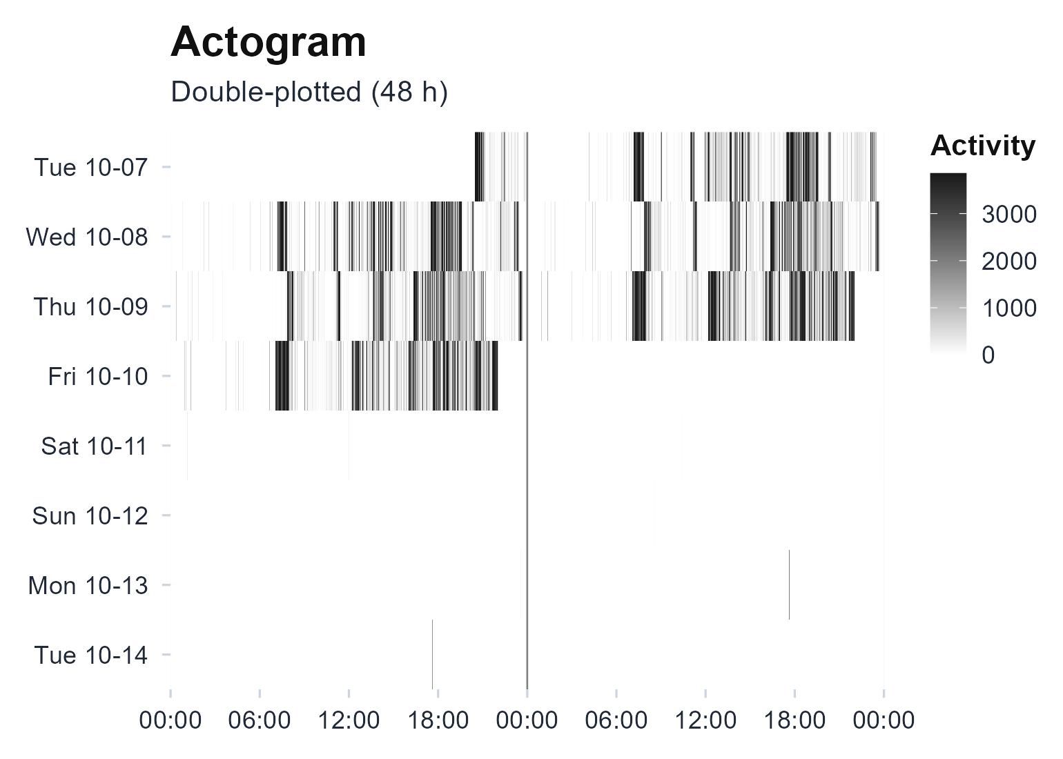
Double-plotted actogram of the bundled recording. The active rows do not stack into one vertical band; they drift, which is the low interdaily stability the metrics report.
The average day makes the L5 and M10 windows concrete: the least-active 5-hour block and the most-active 10-hour block of the folded profile.
plot_profile(agd$axis1, agd$timestamp)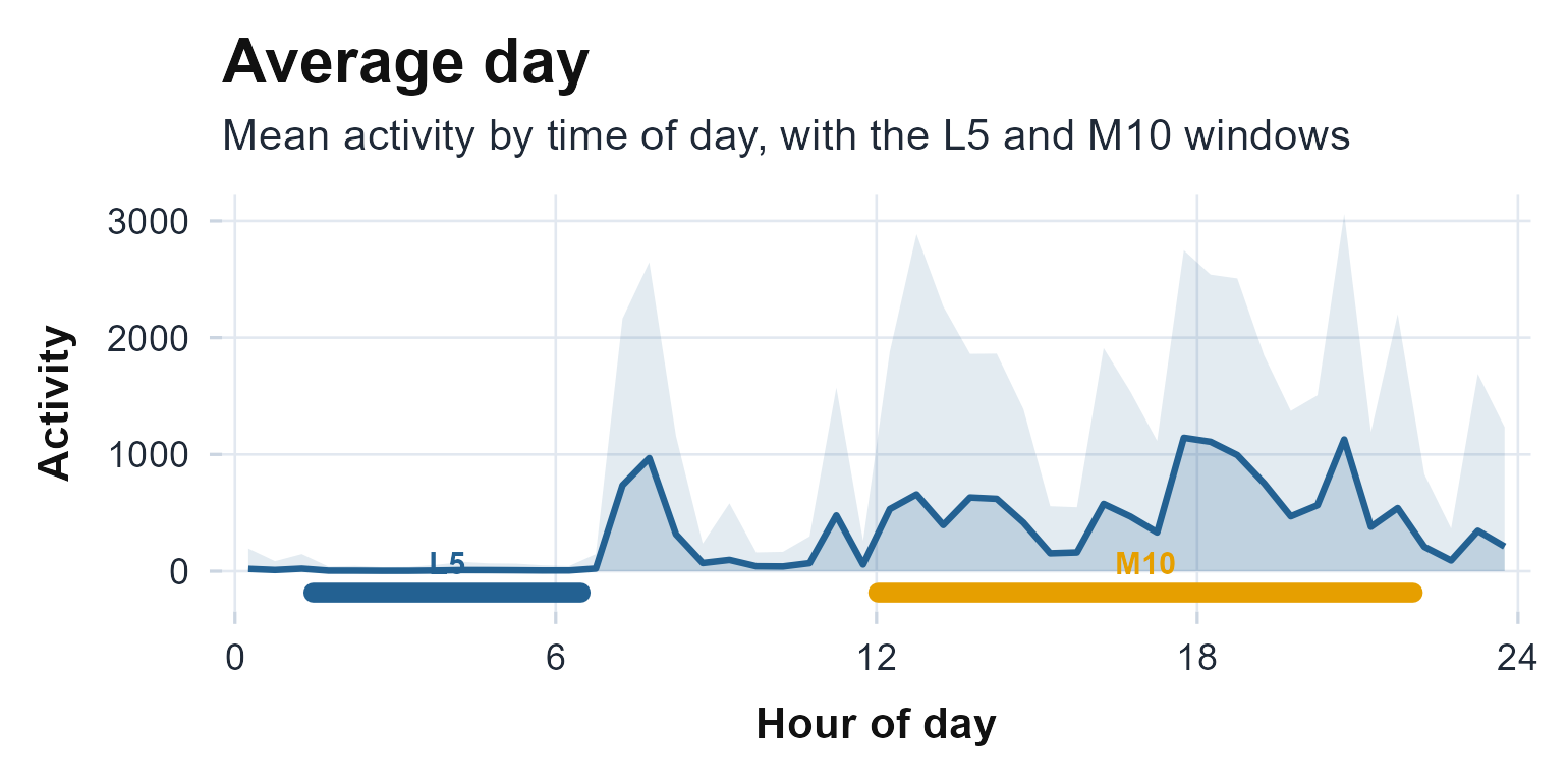
The averaged 24-hour profile (mean with a one-SD band), shading the least-active 5-hour window L5 and the most-active 10-hour window M10.
Reading the numbers
State each metric in human terms:
- IS runs 0 to 1; near 1 is a highly stable 24-hour pattern, below about 0.3 is weak. Here it is low: the days do not land at the same clock time.
- IV runs from about 0 (a smooth sine) to about 2 (noise); above 2 flags a strong ultradian component or a too-short record. The denominator is the data’s own variance, so IV is amplitude-independent.
- RA runs 0 to 1; higher is a stronger day-night contrast.
The most informative reading is often the combination. This recording pairs a high RA (near 0.98) with a low IS (near 0.23): the days are strongly active, but the pattern does not repeat at the same clock time, a strong rhythm carried on irregular timing, which neither number says on its own.
The wider nonparametric family
The same averaged-profile idea generates a family of related descriptors.
Generalising L5/M10 to any window.
activity.extrema() reports the least- and most-active
window of any length, with onset and midpoint times. L1/M1 and L5/M10
are special cases.
activity.extrema(agd$axis1, agd$timestamp, windows = c(1, 5, 10))$table
#>   window_h    L_mean L_onset_h  L_mid_h    M_mean M_onset_h  M_mid_h
#> 1        1  3.102381  2.583333 3.083333 1175.5115  17.71667 18.21667
#> 2        5  6.098095  1.466667 3.966667  756.6825  16.25000 18.75000
#> 3       10 92.392381 21.100000 2.100000  602.9296  12.03333 17.03333
Making the epoch dependence explicit. Because IV and
IS depend on the bin size,
intradaily.variability.multiscale() and
circadian.is.multiscale() recompute them across a range of
epochs and average them into a single IVm and ISm, which vary less
across recordings than the hourly values (Goncalves et al., 2014). IVm spans
1 to 60-minute bins; ISm uses the bin sizes that divide 1440, so each
day splits into whole bins.
intradaily.variability.multiscale(agd$axis1, agd$timestamp)
#> Multiscale Intradaily Variability
#>
#>   IVm (averaged): 0.720
#>
#>  bin_minutes        IV
#>            1 0.5257131
#>            2 0.5902015
#>            3 0.5528503
#>            4 0.5647288
#>            5 0.5345644
#>            6 0.5660806
#>            7 0.5380461
#>            8 0.5610850
#>            9 0.5226812
#>           10 0.5428775
#>           11 0.5247779
#>           12 0.5524045
#>           13 0.5231579
#>           14 0.5636896
#>           15 0.5696848
#>           16 0.5684746
#>           17 0.6280328
#>           18 0.6365006
#>           19 0.6304398
#>           20 0.5888029
#>           21 0.6276416
#>           22 0.5351020
#>           23 0.6802919
#>           24 0.6735950
#>           25 0.6769604
#>           26 0.6602019
#>           27 0.6861135
#>           28 0.7380594
#>           29 0.7154604
#>           30 0.7239887
#>           31 0.6824506
#>           32 0.7538473
#>           33 0.7607380
#>           34 0.8421781
#>           35 0.7227020
#>           36 0.8762168
#>           37 0.7459598
#>           38 0.8316599
#>           39 0.7634351
#>           40 0.7789069
#>           41 0.8080620
#>           42 0.8301316
#>           43 0.9618038
#>           44 0.8420577
#>           45 0.8999159
#>           46 0.8747595
#>           47 0.8542270
#>           48 0.8076128
#>           49 0.9777576
#>           50 0.8028558
#>           51 0.8759503
#>           52 0.7880669
#>           53 0.8529320
#>           54 0.9957456
#>           55 0.8135647
#>           56 0.9072522
#>           57 0.9750063
#>           58 0.8813777
#>           59 0.8670441
#>           60 0.8360881
circadian.is.multiscale(agd$axis1, agd$timestamp)
#> Multiscale Interdaily Stability
#>
#>   ISm (averaged): 0.210
#>
#>  bin_minutes     IS
#>            1 0.1827
#>            2 0.1874
#>            3 0.1912
#>            4 0.1946
#>            5 0.1950
#>            6 0.1984
#>            8 0.2024
#>            9 0.2044
#>           10 0.2042
#>           12 0.2079
#>           15 0.2102
#>           16 0.2163
#>           18 0.2101
#>           20 0.2157
#>           24 0.2188
#>           30 0.2238
#>           32 0.2247
#>           36 0.2193
#>           40 0.2250
#>           45 0.2365
#>           48 0.2296
#>           60 0.2279
plot_multiscale(agd$axis1, agd$timestamp)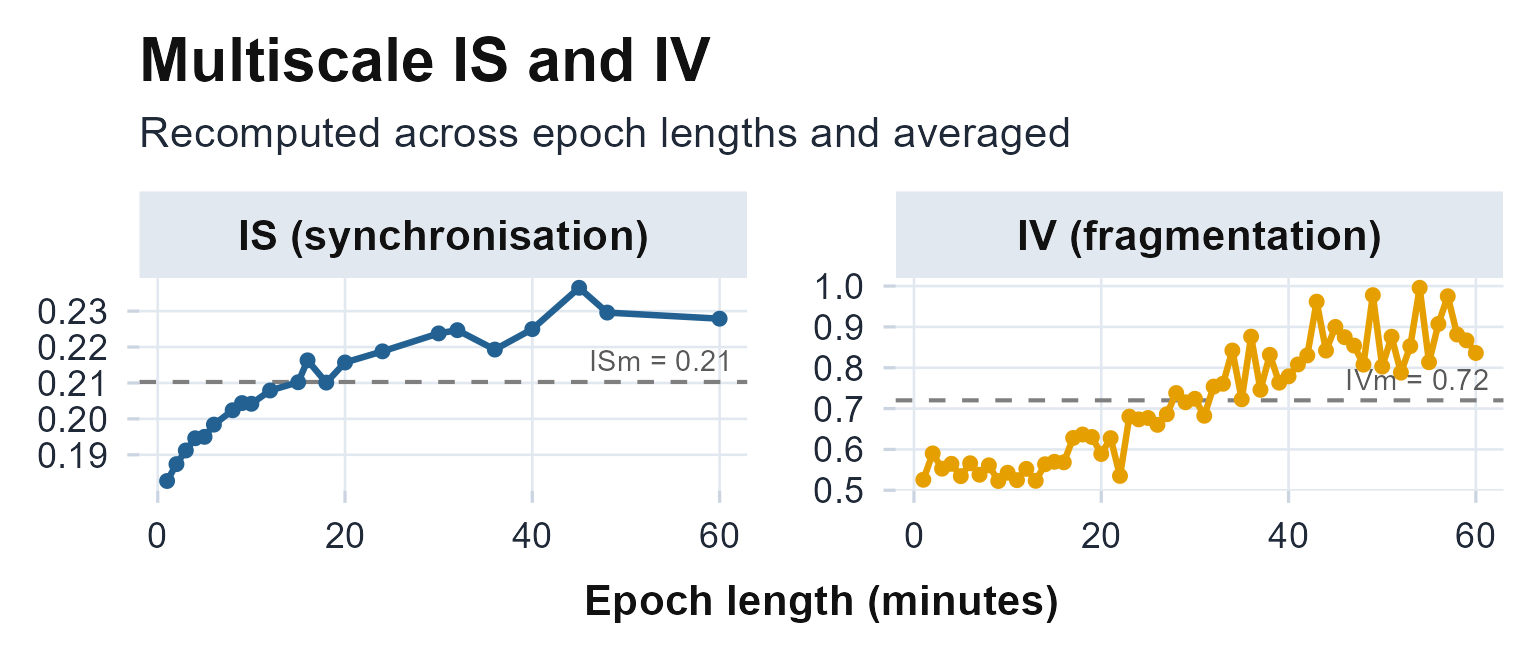
IS and IV across epoch lengths, with the averaged ISm and IVm (dashed). Both vary less across recordings than a single hourly value.
How cleanly rest separates from activity. The dichotomy index I<O is the percentage of rest-span counts that fall below the median of the active-span counts (Mormont et al., 2000): where is the median active-span count. A high I<O means rest is quiet relative to the active day. Here we mark the night hours as rest.
h <- as.numeric(format(agd$timestamp, "%H"))
dichotomy.index(agd$axis1, rest = h >= 23 | h < 7)
#> Dichotomy Index (I<O)
#>
#>   I<O:             0.0%
#>   Active median:   0.0 counts
#>   Rest / active epochs: 3360 / 6559
plot_dichotomy(agd$axis1, rest = h >= 23 | h < 7)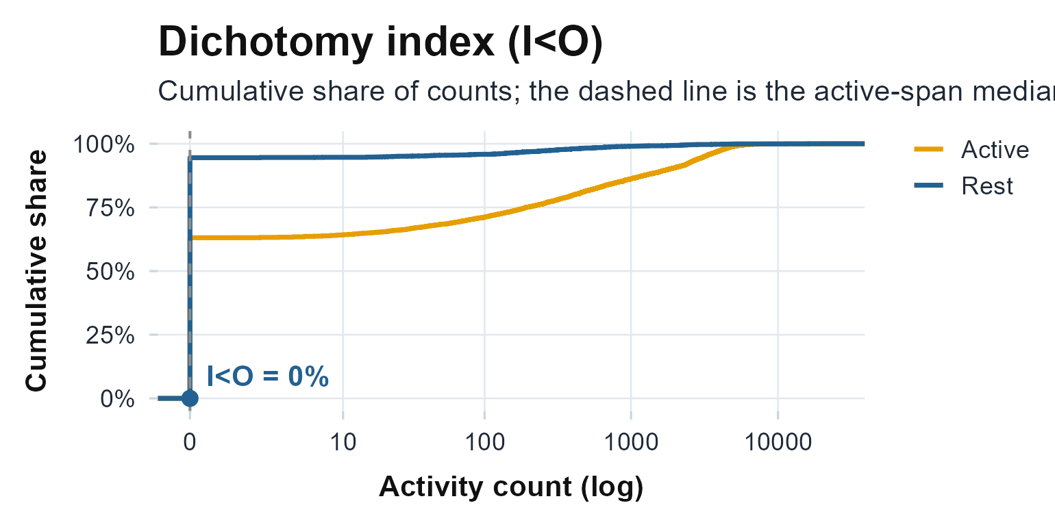
Rest-span and active-span count distributions. A high I<O means most rest-span counts fall below the active-span median (dashed).
On this recording the active-span count median is zero, so the strict I < median comparison collapses to 0 percent. The dichotomy index needs a denser active span, a coarser epoch or a count threshold in place of the median, to separate quiet rest from an active day; it is a caution worth keeping for sparse minute-level counts.
Fragmentation. state.transitions()
gives the kRA and kAR rates, the rest-to-active and active-to-rest
probabilities read off the plateau of the bout-length survival curve
(Lim et al.,
2011). transition.probability() gives the
maximum-likelihood and Bayesian transition probabilities of Danilevicz et al. (2024), taken straight from the
epoch-to-epoch transition counts. Both capture fragmentation a single
amplitude cannot.
state.transitions(agd$axis1)
#> Rest-Activity State Transitions
#>
#>   Threshold:  >= 1 counts = active
#>   kRA (rest->active): 0.0392   (356 rest bouts)
#>   kAR (active->rest): 0.1068   (356 active bouts)
#>   pRA / pAR:          0.0487 / 0.1367
transition.probability(agd$axis1)[c("tp_ra_mle", "tp_ar_mle")]
#> $tp_ra_mle
#> [1] 0.04854369
#>
#> $tp_ar_mle
#> [1] 0.1366603
plot_transitions(agd$axis1)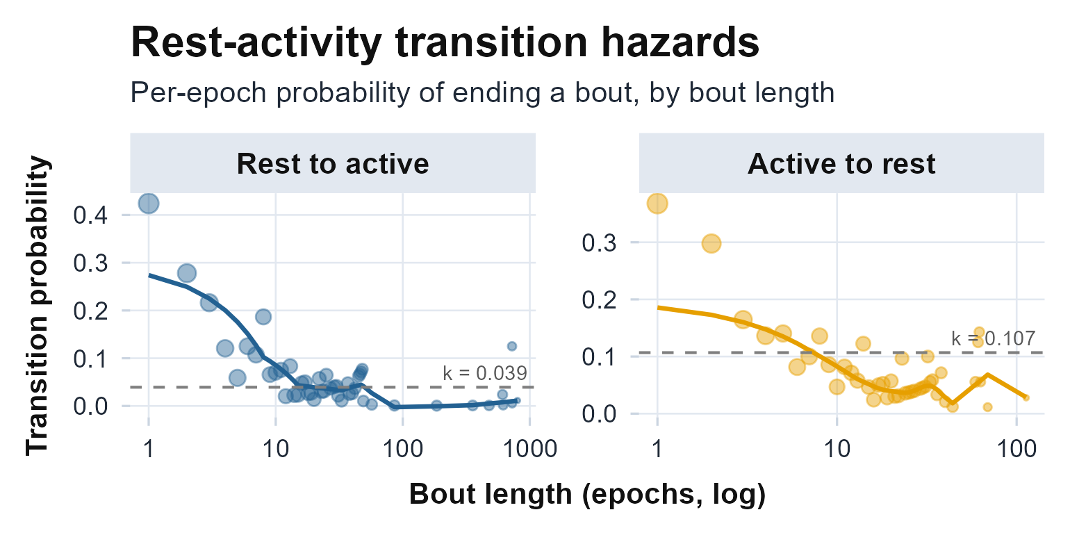
Transition hazards versus bout length, with a LOWESS fit and the sustained rates kRA and kAR (dashed).
Per day, to see drift.
circadian.daily() reports each day on its own, so
within-recording change shows instead of being averaged away.
daily <- circadian.daily(agd$axis1, agd$timestamp)$daily
ggplot(daily, aes(date, M10_onset_h)) +
  geom_line(colour = "grey60") + geom_point(colour = "#236192", size = 2) +
  labs(x = NULL, y = "M10 onset (h)") +
  theme_actiRhythm()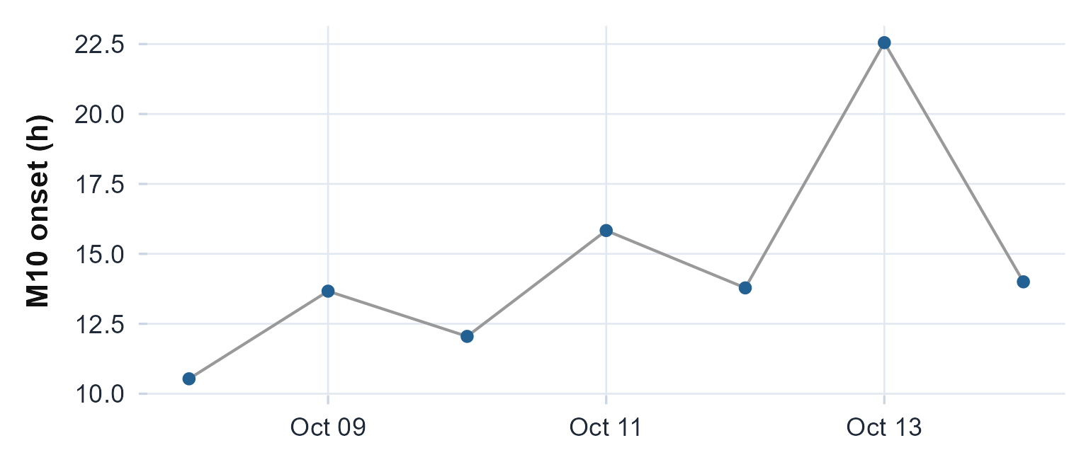
The most-active-window onset for each day. Reporting it per day, rather than pooled, shows how steady the active phase is.
Limitations
- Missing data moves the numbers. A few device-off days can shift IS as much as a real change; always check coverage and gate on wear time.
- Epoch dependence. Compare IV (and to a lesser extent IS) only across records binned to the same epoch; use the multiscale view when epochs differ.
- A minimum of valid days. Very short records give unstable IS; the function enforces a per-day validity threshold and reports how many days qualified.
Reference and validation
The nonparametric battery follows Witting et
al. (1990) and Van Someren et al. (1999), with the multiscale and
dichotomy extensions of Goncalves et al. (2014) and Mormont et al. (2000), and the fragmentation rates of
Lim et al. (2011) and Danilevicz et al. (2024). actiRhythm’s IS, IV, RA,
L5, and M10 are cross-checked against the nparACT and
ActCR reference implementations (to the printed precision)
in the Validation article and the
package’s test suite.