
The idea, and a rule to remember
The cosinor fits a cosine of fixed period to the rest-activity rhythm and reads three interpretable numbers off it: the MESOR (the rhythm-adjusted mean), the amplitude (half the peak-to-trough swing), and the acrophase (the clock time of the peak). Where the nonparametric metrics make no shape assumption, the cosinor makes a strong one (a single, symmetric sinusoid) and in return gives you parameters you can model and compare across people.
The rule to carry through this article: a significant rhythmicity test tells you the rhythm is not flat, not that a single cosine is the right shape. Always read the percent-rhythm alongside the p-value; it is how much of the daily structure the one cosine actually captures, and a low value is the data telling you the shape is wrong.
The math
Write the averaged daily activity as at clock time , with period (24 hours by default) and . The cosinor model is
which is fitted in its linear form
so the three parameters come straight from the regression coefficients:
The reported acrophase is the clock time of the peak, reduced to . The fit uses the averaged hour-of-day profile, so the zero-amplitude F-test of (Nelson et al., 1979) and the percent-rhythm (Cornelissen, 2014) are computed on the profile hours present (the F-test denominator is hours , not the raw epoch count).
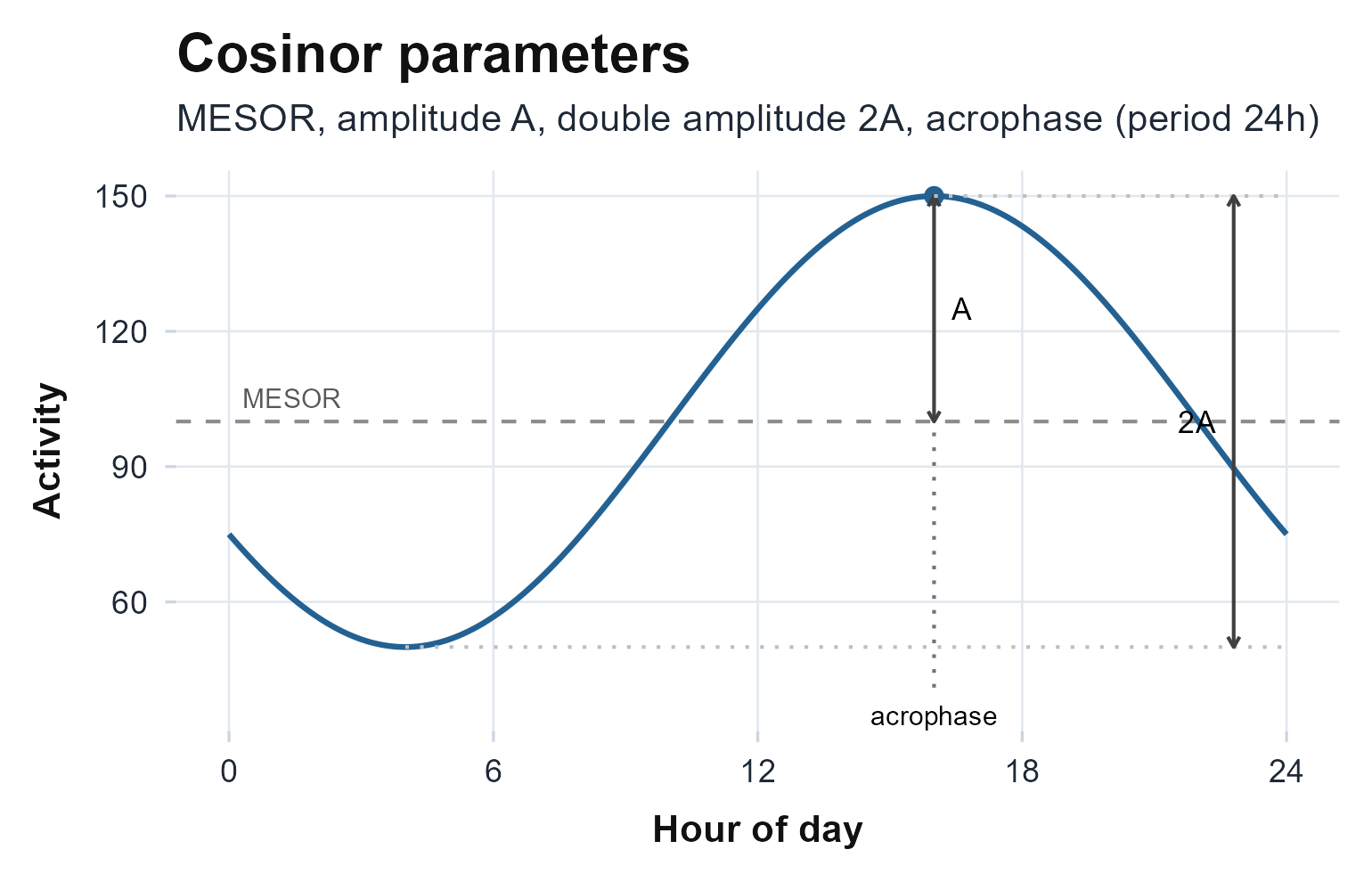
The cosinor parameters: the MESOR midline, the amplitude A and double amplitude 2A, and the acrophase as the clock time of the peak.
Assumptions, and when they break
- One symmetric sinusoid. The model has a single peak and trough of equal, smooth shape. Asymmetric days (a fast morning rise, a slow evening decline), squared-off days, naps, and bimodal patterns all violate it. The section “When a single cosine is the wrong shape” below makes this concrete.
- A fixed, known period. The cosinor assumes ; it does not estimate it. If the rhythm may be free-running, estimate the period first (see Choosing a method).
- The acrophase is only meaningful once the amplitude is. A clock time of the peak is uninterpretable if the amplitude is not distinguishable from zero.
Recovering known truth
First, see the fit recover parameters we plant. We build a seven-day recording from a cosine with a MESOR of 200, an amplitude of 100, and a 16:00 acrophase, then add noise.
ts <- seq(as.POSIXct("2024-01-01", tz = "UTC"), by = 60, length.out = 7 * 1440)
th <- as.numeric(difftime(ts, ts[1], units = "hours"))
set.seed(1)
known <- pmax(0, 200 + 100 * cos(2 * pi * (th - 16) / 24) + rnorm(length(ts), 0, 15))

ca <- cosinor.analysis(known, ts)
knitr::kable(
  data.frame(parameter = c("MESOR", "amplitude", "acrophase (h)"),
             planted   = c(200, 100, 16),
             recovered = c(ca$mesor, ca$amplitude, ca$acrophase)),
  digits = 2, caption = "The cosinor recovers the planted MESOR, amplitude, and acrophase."
)| parameter | planted | recovered | |
|---|---|---|---|
| MESOR | 200 | 199.90 | |
| cos_term | amplitude | 100 | 99.36 |
| sin_term | acrophase (h) | 16 | 16.01 |
The rhythmicity test confirms the rhythm is real and reports how much of the variance the cosine carries.
rt <- rhythmicity.test(known, ts, cosinor_result = ca)
c(F = rt$F, p_value = rt$p_value, percent_rhythm = rt$percent_rhythm, rhythmic = rt$rhythmic)
#>              F        p_value percent_rhythm       rhythmic
#>   1.049895e+05   1.000000e-42   9.999000e+01   1.000000e+00
On a real recording
The bundled recording runs the same way.
cosinor.analysis() returns a typed object;
rhythmicity.test() checks whether the rhythm is
statistically real.
agd <- agd.counts(read.agd(example_agd(1), verbose = FALSE))
cos <- cosinor.analysis(agd$axis1, agd$timestamp, period = 24)
c(mesor = unname(cos$mesor), amplitude = unname(cos$amplitude),
  acrophase = unname(cos$acrophase), r_squared = unname(cos$r_squared))
#>     mesor amplitude acrophase r_squared
#>  327.2500  295.6300   16.9200    0.4371
rhythmicity.test(agd$axis1, agd$timestamp, cosinor_result = cos)
#> Cosinor Rhythmicity Test (Halberg zero-amplitude F-test)
#>
#> H0: amplitude = 0 (no rhythm)
#>   Period:         24 h
#>   F(2, 21):        8.15
#>   P-value:        0.0024
#>   Percent rhythm: 43.7% (R-squared = 0.4371)
#>   Rhythmic:       YES (alpha = 0.05)
plot_extended_cosinor(agd$axis1, agd$timestamp)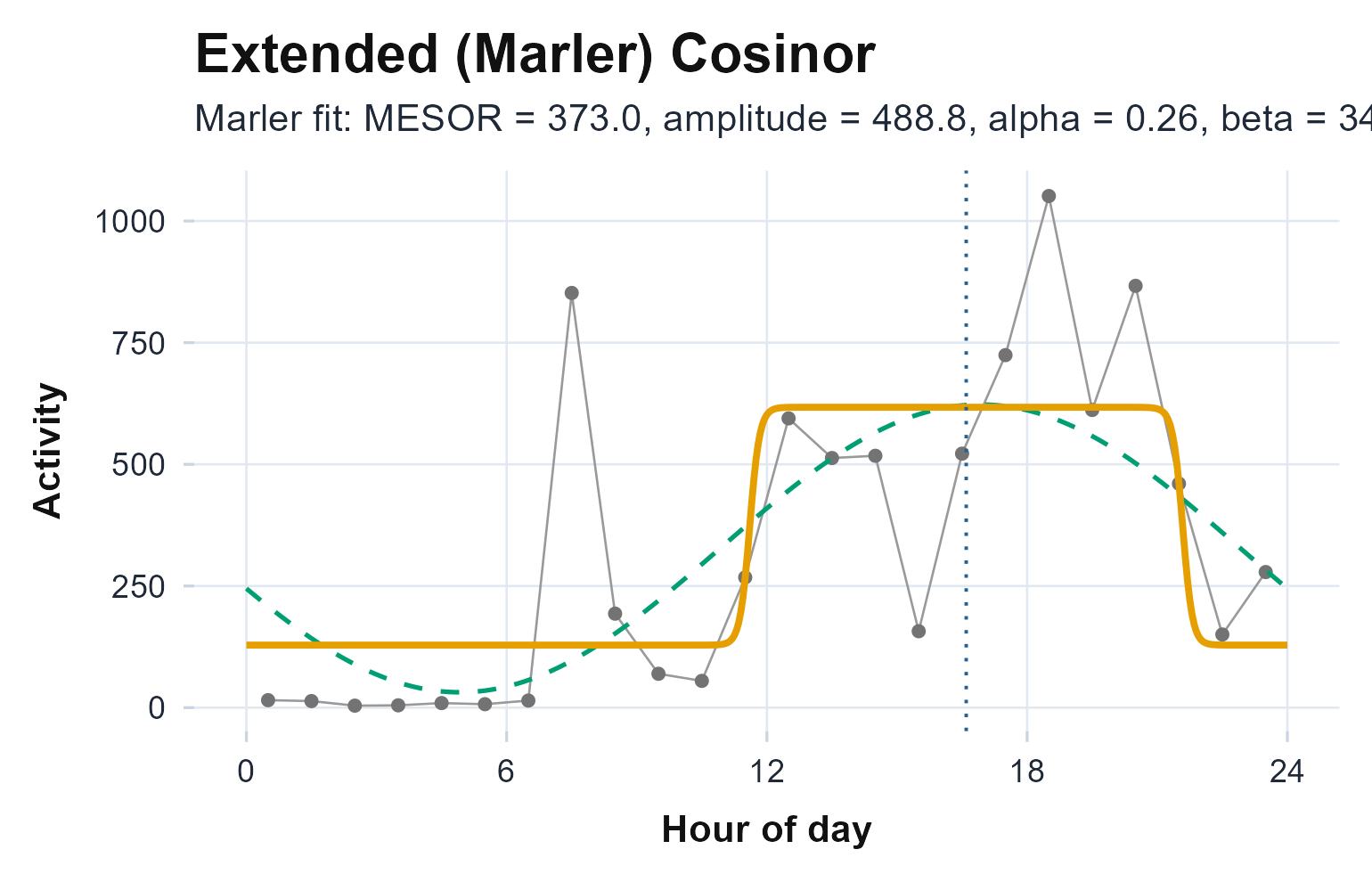
The averaged hourly profile with two fits overlaid: the ordinary single cosine (dashed) and the extended Marler fit (orange), which allows squared-off peaks. Where the points leave the single cosine is the structure it cannot follow; the Marler fit is covered under the wider cosinor family below.
For the joint uncertainty in amplitude and acrophase,
cosinor.confidence.ellipse() returns the Bingham et al. (1982) ellipse; an ellipse that
excludes the origin is the geometric form of “a detectable rhythm”.
el <- cosinor.confidence.ellipse(cos)
c(excludes_origin = el$excludes_origin, rhythm_detected = el$rhythm_detected)
#> excludes_origin rhythm_detected
#>            TRUE            TRUE
plot_cosinor_ellipse(agd$axis1, agd$timestamp)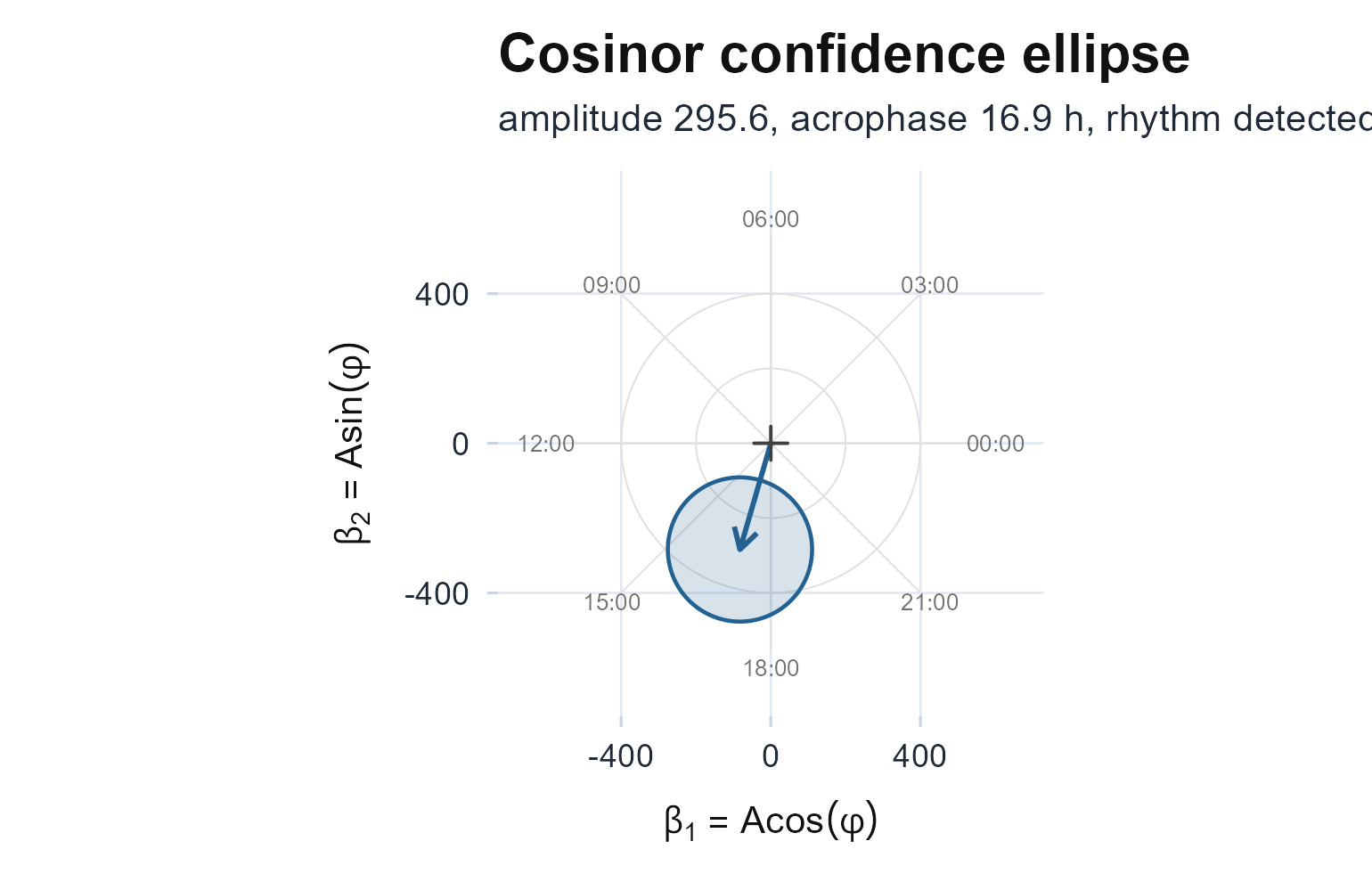
The amplitude-acrophase confidence ellipse on the clock plane. The arrow is the (amplitude, acrophase) estimate measured from the origin; because the ellipse excludes the origin, the rhythm is detectable.
Reading the numbers
- MESOR is the rhythm-adjusted mean, the midline of the fitted cosine rather than the raw average.
- Amplitude is half the peak-to-trough swing; larger is a stronger sinusoidal component.
- Acrophase is the clock time of the peak and is circular: 23.5 and 0.5 are an hour apart, not 23, and it is interpretable only once the amplitude is clearly non-zero.
- Percent-rhythm is the share of variance the cosine explains; a low value next to a small p-value is the warning the rule above flags.
When a single cosine is the wrong shape
This is the rule in action. We build a siesta day (an active morning and evening with a midday dip), which has a clear 24-hour rhythm but is not a single symmetric cosine.
hod <- as.numeric(format(ts, "%H")) + as.numeric(format(ts, "%M")) / 60
set.seed(2)
siesta <- pmax(0, 120 + 60 * cos(2 * pi * 2 * (hod - 9.5) / 24) -   # twin morning/evening peaks
                    45 * cos(2 * pi * (hod - 3) / 24) +             # carves the midday dip
                    rnorm(length(ts), 0, 12))

cs  <- cosinor.analysis(siesta, ts)
rts <- rhythmicity.test(siesta, ts, cosinor_result = cs)
c(rhythmic = rts$rhythmic, p_value = rts$p_value, percent_rhythm = rts$percent_rhythm)
#>       rhythmic        p_value percent_rhythm
#>    1.000000000    0.008707296   36.350000000
The test is significant (the rhythm is not flat), yet the single cosine explains only about 37 percent of the day. It cannot bend to the twin morning and evening peaks with the midday dip between them. A multi-harmonic fit recovers the shape: it selects two components and explains essentially all of it (the chunk below reports the R-squared).
mc <- cosinor.multicomponent(siesta, ts)
c(n_harmonics = mc$n_harmonics, r_squared = mc$r_squared)
#> n_harmonics   r_squared
#>    2.000000    0.999903
mc$harmonics
#>    harmonic amplitude acrophase_h
#> x2        1  44.72900   15.016326
#> x4        2  59.18037    9.506901
plot_multicomponent(siesta, ts)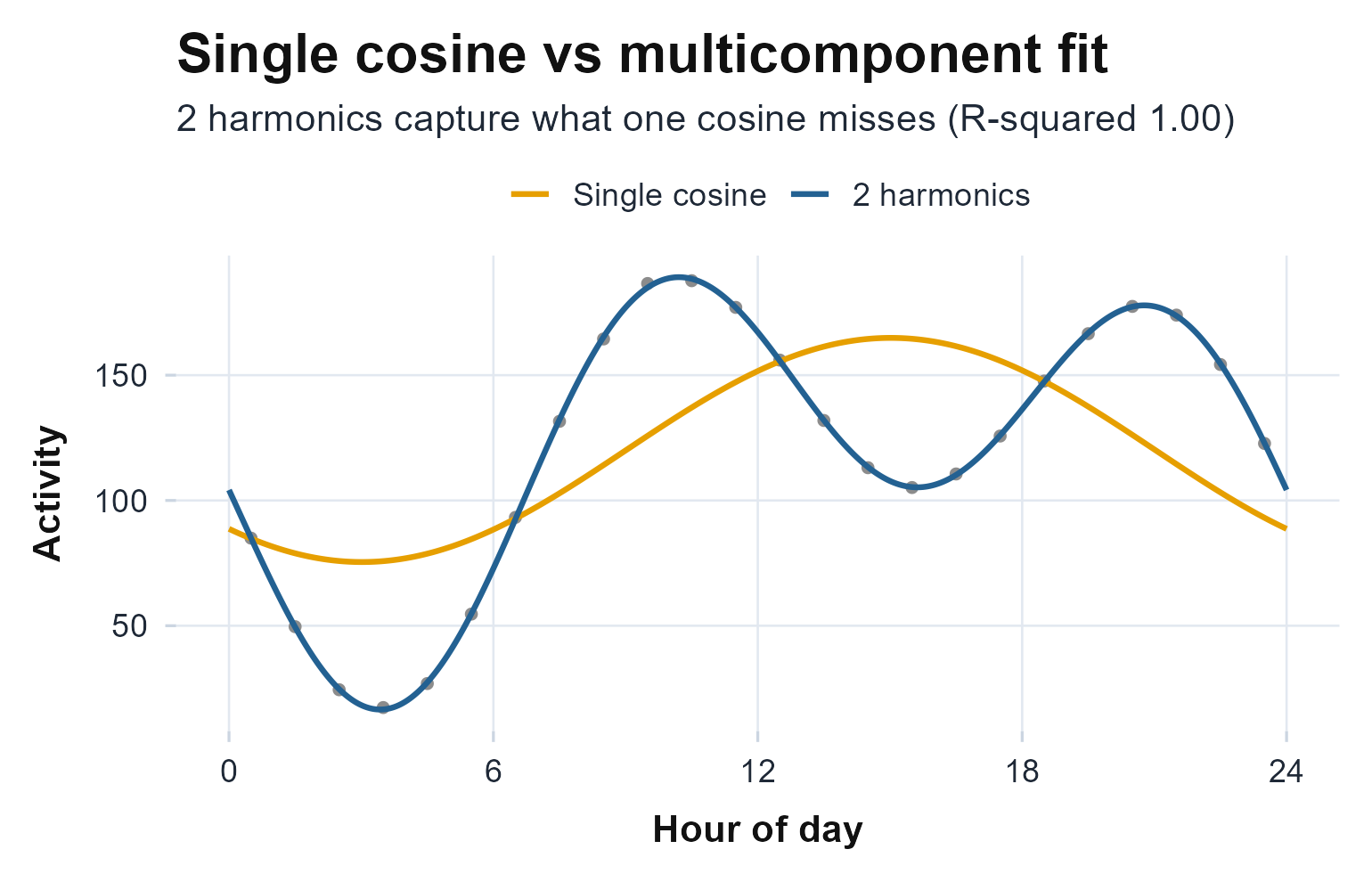
The single cosine (orange) misses the midday dip; the two-harmonic fit (blue) recovers it.
So in practice, let the low percent-rhythm, not the significant p-value, send you to a richer model rather than a misleading single acrophase.
The wider cosinor family
-
Asymmetric and squared-off days:
cosinor.antilogistic()fits the sigmoidally transformed cosine of Marler et al. (2006), adding shape parameters (steepness, up- and down-mesor times) the single cosinor lacks.
fit <- cosinor.antilogistic(agd$axis1, agd$timestamp)
c(MESOR = fit$MESOR, amplitude = fit$amplitude, acrophase = fit$acrophase,
  UpMesor = fit$UpMesor, DownMesor = fit$DownMesor)
#>     MESOR amplitude acrophase   UpMesor DownMesor
#> 372.95566 488.79342 16.59496 11.60451 21.58541-
Several harmonics:
cosinor.extended()andcosinor.multicomponent()fit the multi-component (harmonic) cosinor of Cornelissen (2014) for non-sinusoidal days;cosinor.multicomponent()chooses the number of components by AIC or BIC. -
The parametric amplitude as a ratio:
circadian.quotient()turns the cosinor amplitude and MESOR into the circadian quotient (amplitude / MESOR). -
Pooling the evidence:
consensus.rhythmicity()runs the cosinor F-test, the Lomb-Scargle false-alarm probability, and the chi-square periodogram, and reports a majority vote with a Cauchy-combined p-value (valid although the tests share one series). -
From one subject to a group:
population.cosinor()pools per-subject fits into a Bingham population-mean rhythm with confidence intervals, andcosinor.compare()tests whether the rhythm differs between two groups with the Bingham amplitude-acrophase Hotelling , a separate MESOR test, and auxiliary per-parameter comparisons (Bingham et al., 1982). See Choosing a method for when to reach for each.
Limitations
- The period is assumed, not estimated. Set it correctly, or estimate it first with the periodograms.
- A single component is symmetric. Real days rarely are; read the percent-rhythm and escalate to the extended or multicomponent fit when it is low.
- The acrophase needs a real amplitude. Report it only when the amplitude is clearly distinguishable from zero (the rhythmicity test and the confidence ellipse are the checks).
Reference and validation
The cosinor follows Cornelissen (2014) with the zero-amplitude
test of Nelson et al. (1979), the anti-logistic extension of
Marler et al. (2006), and the population framework of
Bingham et al. (1982). actiRhythm’s single and
extended cosinor are cross-checked against the cosinor
package and ActCR::ActExtendCosinor (to the printed
precision) in the Validation article and
the package’s test suite.