
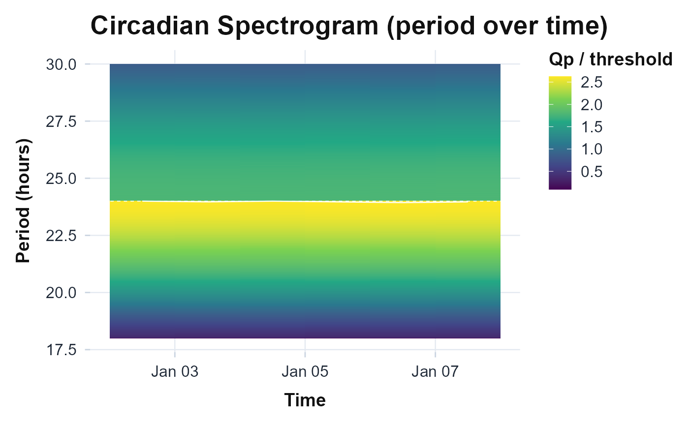
Slides a window across the recording and computes the chi-square (Sokolove-Bushell) periodogram in each window, producing a period-by-time map that shows how the dominant period and its strength drift across the recording (non-stationarity, fragmentation, re-entrainment). A single global periodogram or cosinor fit cannot show this.
Usage
circadian.spectrogram(
  counts,
  timestamps,
  window_hours = 72,
  step_hours = 6,
  from = 18,
  to = 30,
  epoch_length = NULL
)
Arguments
- counts
Numeric activity vector.
- timestamps
POSIXct timestamps, one per value.
- window_hours
Sliding-window length in hours (default 72).
- step_hours
Step between successive windows in hours (default 6).
- from, to
Period search window in hours (default 18, 30).
- epoch_length
Epoch length in seconds (default 60).
Value
An object of class actiRhythm_spectrogram: a long data
frame (window centre time, period, power) and a ggplot heat map in
$plot.
Examples
# \donttest{
t_hours <- seq(0, 8 * 24, by = 1 / 60)
ts <- as.POSIXct("2024-01-01", tz = "UTC") + t_hours * 3600
counts <- 100 + 80 * cos(2 * pi * t_hours / 24) + rnorm(length(t_hours), 0, 20)
circadian.spectrogram(counts, ts, step_hours = 24)$plot
 # }
# }