Plot the Detrended Fluctuation Analysis (DFA) Scaling Relationship

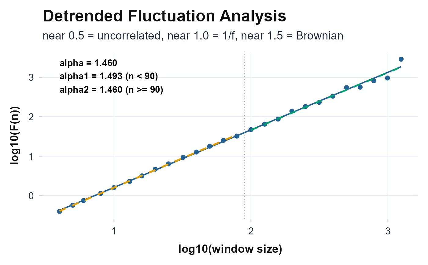
Runs fractal.dfa on an activity series and draws the detrended-fluctuation log-log scaling plot: log10(F(n)) against log10(n) (window size). A regression line whose slope is the overall scaling exponent alpha is overlaid, and when the analysis splits the scales at a breakpoint the short- (alpha1) and long-timescale (alpha2) segments are drawn separately. The exponents are annotated on the plot and an interpretive guide appears in the subtitle.

Usage

plot_dfa(counts)

Arguments

counts: Numeric vector of activity counts (minute-level recommended). The longest continuous non-NA segment is analyzed internally by fractal.dfa().

Value

A ggplot object: log10(F(n)) (y) versus log10(window size) (x) as points with fitted scaling line(s) and alpha/alpha1/alpha2 annotations. On an unusable series (too short, all-NA, or constant) an annotated empty ggplot is returned. The function never errors.

Details

DFA quantifies long-range temporal correlations. The scaling exponent is the slope of log10(F(n)) regressed on log10(n): alpha near 0.5 indicates uncorrelated (white) noise, alpha near 1.0 indicates 1/f (pink) noise, and alpha near 1.5 indicates Brownian (random-walk) noise. The scales, fluctuations, alpha, alpha1, alpha2 and breakpoint_min fields returned by fractal.dfa() drive the plot directly.

References

Peng CK, Buldyrev SV, Havlin S, Simons M, Stanley HE, Goldberger AL (1994). “Mosaic organization of DNA nucleotides.” Physical Review E, 49(2), 1685–1689. doi:10.1103/PhysRevE.49.1685 .

Hu K, Van Someren EJW, Shea SA, Scheer FAJL (2009). “Reduction of scale invariance of activity fluctuations with aging and Alzheimer's disease: Involvement of the circadian pacemaker.” Proceedings of the National Academy of Sciences, 106(8), 2490–2494. doi:10.1073/pnas.0806087106 .

Examples

# \donttest{
set.seed(1)
plot_dfa(cumsum(rnorm(5000)))   # Brownian-like, alpha near 1.5

# }