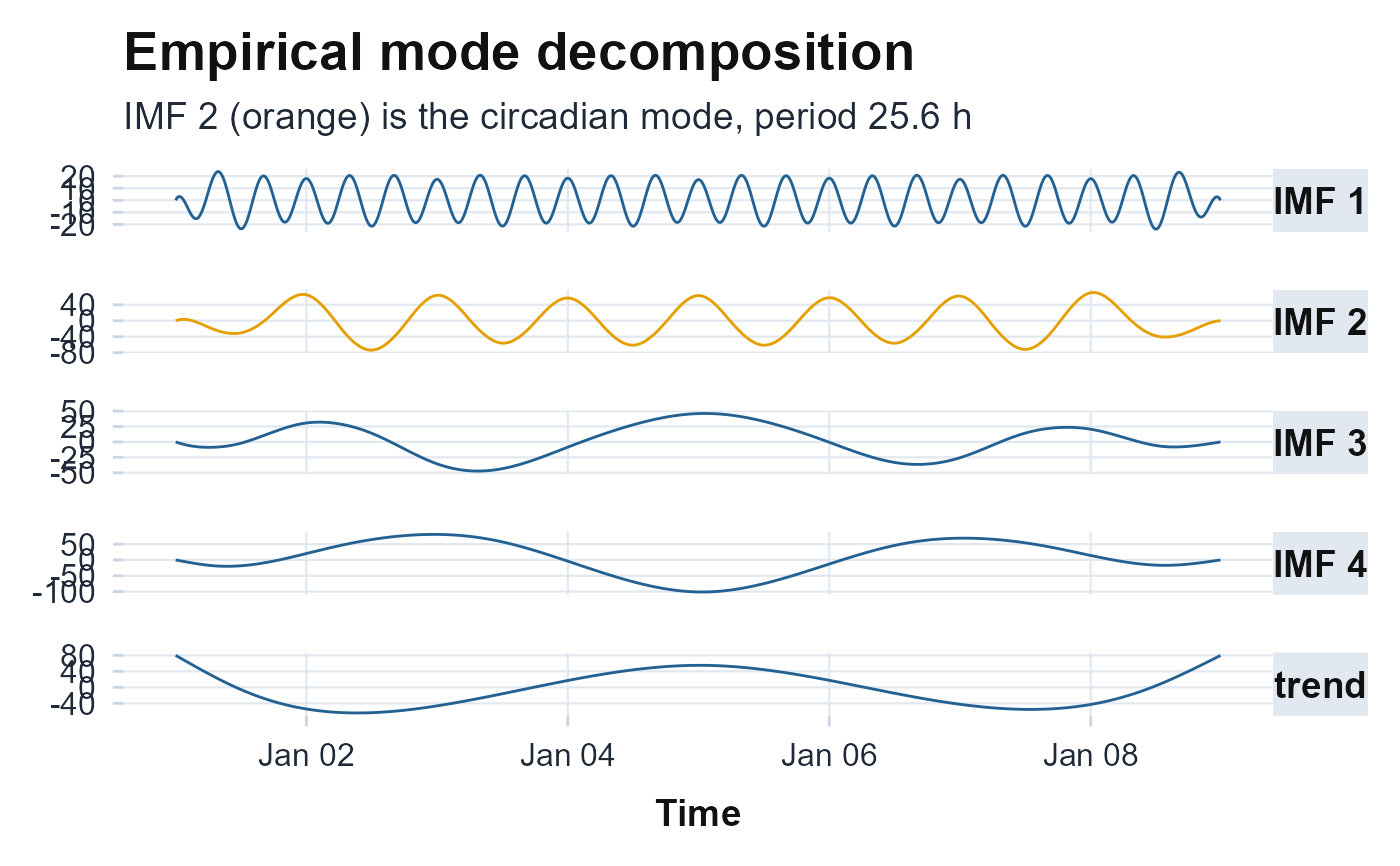
Empirical Mode Decomposition Stack — plot

Stacks the intrinsic mode functions and residual trend from circadian.emd, finest at the top to the trend at the bottom, over a shared time axis, with the circadian IMF highlighted. Returns a ggplot object and never errors.

Usage

plot_emd(counts, timestamps, ensemble = 1L, epoch_length = 60)

Arguments

counts: Numeric activity vector.
timestamps: POSIXct timestamps, one per value.
ensemble: Ensemble size for EEMD (default 1 = plain EMD).
epoch_length: Epoch length in seconds (default 60).

Value

A ggplot object.

References

Huang NE, Shen Z, Long SR, Wu MC, Shih HH, Zheng Q, Yen NC, Tung CC, Liu HH (1998). “The empirical mode decomposition and the Hilbert spectrum for nonlinear and non-stationary time series analysis.” Proceedings of the Royal Society A, 454(1971), 903–995. doi:10.1098/rspa.1998.0193 .

Examples

# \donttest{
ts <- seq(as.POSIXct("2024-01-01", tz = "UTC"), by = 600, length.out = 8 * 144)
th <- as.numeric(difftime(ts, ts[1], units = "hours"))
plot_emd(100 + 60 * cos(2 * pi * th / 24) + 20 * cos(2 * pi * th / 8), ts, epoch_length = 600)

# }