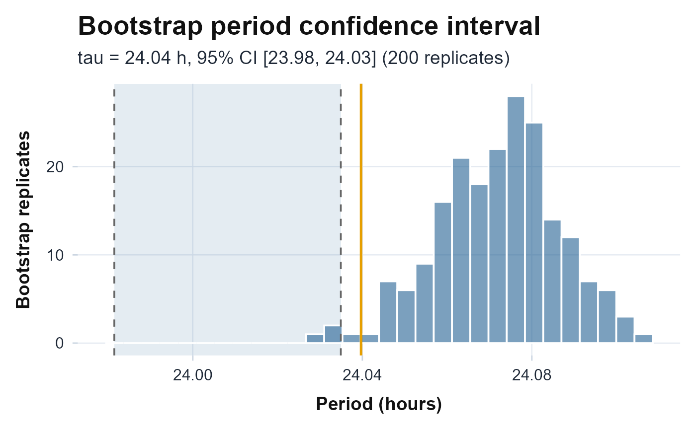
Bootstrap Period Confidence Interval — plot_period

Shows the distribution of bootstrap replicate periods from period.ci with the point estimate and the confidence-interval band marked, so the period estimate is read together with its uncertainty. Returns a ggplot object and never errors.

Usage

plot_period_ci(
  counts,
  timestamps,
  from = 18,
  to = 30,
  level = 0.95,
  n_boot = 200,
  seed = NULL
)

Arguments

counts: Numeric activity vector.
timestamps: POSIXct timestamps, one per value.
from, to: Period search window in hours (default 18, 30).
level: Confidence level (default 0.95).
n_boot: Bootstrap replicates (default 200).
seed: Optional RNG seed for reproducibility.

Value

A ggplot object.

References

Kunsch HR (1989). “The jackknife and the bootstrap for general stationary observations.” The Annals of Statistics, 17(3), 1217–1241. doi:10.1214/aos/1176347265 .

Politis DN, Romano JP (1992). “A circular block-resampling procedure for stationary data.” In LePage R, Billard L (eds.), Exploring the Limits of Bootstrap, 263–270. Wiley, New York.

Examples

# \donttest{
ts <- seq(as.POSIXct("2024-01-01", tz = "UTC"), by = 60, length.out = 7 * 1440)
h  <- as.numeric(format(ts, "%H"))
plot_period_ci(100 + 60 * cos(2 * pi * (h - 8) / 24) + rnorm(length(ts), 0, 20), ts)

# }