Wavelet Power Scalogram

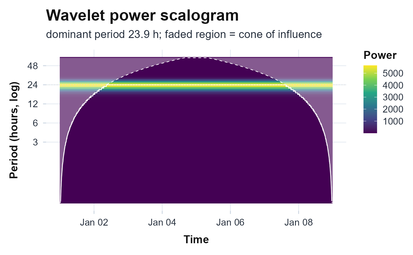
Draws the Morlet wavelet power surface from circadian.wavelet: time on the x-axis, period (hours, log scale) on the y, scale-rectified power as the fill, with the cone of influence faded out, the per-time dominant-period ridge traced, and the 24-hour reference marked. Returns a ggplot object and never errors.

Usage

plot_wavelet(counts, timestamps, epoch_length = 60)

Arguments

counts

Numeric activity vector.

timestamps

POSIXct timestamps, one per value.

epoch_length

Epoch length in seconds (default 60).

Value

A ggplot object.

References

Torrence C, Compo GP (1998). “A practical guide to wavelet analysis.” Bulletin of the American Meteorological Society, 79(1), 61–78. doi:10.1175/1520-0477(1998)079<0061:APGTWA>2.0.CO;2 .

Leise TL (2013). “Wavelet analysis of circadian and ultradian behavioral rhythms.” Journal of Circadian Rhythms, 11, 5. doi:10.1186/1740-3391-11-5 .

Examples

# \donttest{
ts <- seq(as.POSIXct("2024-01-01", tz = "UTC"), by = 600, length.out = 8 * 144)
th <- as.numeric(difftime(ts, ts[1], units = "hours"))
plot_wavelet(100 + 80 * cos(2 * pi * th / 24), ts, epoch_length = 600)

# }